Terminals are shown in bold font and nonterminals in italics. Literal characters are given in single quotes. Parentheses ( and ) indicate grouping when needed. Square brackets [ and ] enclose optional items. Vertical bars | separate alternatives.

graph	:	[ strict ] (graph \| digraph) [ ID ] '{' stmt_list '}'
stmt_list	:	[ stmt [ ';' ] stmt_list ]
stmt	:	node_stmt
	\|	edge_stmt
	\|	attr_stmt
	\|	ID '=' ID
	\|	subgraph
attr_stmt	:	(graph \| node \| edge) attr_list
attr_list	:	'[' [ a_list ] ']' [ attr_list ]
a_list	:	ID '=' ID [ (';' \| ',') ] [ a_list ]
edge_stmt	:	(node_id \| subgraph) edgeRHS [ attr_list ]
edgeRHS	:	edgeop (node_id \| subgraph) [ edgeRHS ]
node_stmt	:	node_id [ attr_list ]
node_id	:	ID [ port ]
port	:	':' ID [ ':' compass_pt ]
	\|	':' compass_pt
subgraph	:	[ subgraph [ ID ] ] '{' stmt_list '}'
compass_pt	:	(n \| ne \| e \| se \| s \| sw \| w \| nw \| c \| _)

The keywords node, edge, graph, digraph, subgraph, and strict are case-independent. Note also that the allowed compass point values are not keywords, so these strings can be used elsewhere as ordinary identifiers and, conversely, the parser will actually accept any identifier.

An ID is one of the following:

Any string of alphabetic ([a-zA-Z\200-\377]) characters, underscores ('_') or digits([0-9]), not beginning with a digit;
a numeral [-]^?(.[0-9]⁺ | [0-9]⁺(.[0-9]^*)^? );
any double-quoted string ("...") possibly containing escaped quotes (\")¹;
an HTML string (<...>).

An ID is just a string; the lack of quote characters in the first two forms is just for simplicity. There is no semantic difference between abc_2 and "abc_2", or between 2.34 and "2.34". Obviously, to use a keyword as an ID, it must be quoted. Note that, in HTML strings, angle brackets must occur in matched pairs, and newlines and other formatting whitespace characters are allowed. In addition, the content must be legal XML, so that the special XML escape sequences for ", &, <, and > may be necessary in order to embed these characters in attribute values or raw text. As an ID, an HTML string can be any legal XML string. However, if used as a label attribute, it is interpreted specially and must follow the syntax for HTML-like labels.

Both quoted strings and HTML strings are scanned as a unit, so any embedded comments will be treated as part of the strings.

An edgeop is -> in directed graphs and -- in undirected graphs.

The language supports C++-style comments: /* */ and //. In addition, a line beginning with a '#' character is considered a line output from a C preprocessor (e.g., # 34 to indicate line 34 ) and discarded.

Semicolons and commas aid readability but are not required. Also, any amount of whitespace may be inserted between terminals.

As another aid for readability, dot allows double-quoted strings to span multiple physical lines using the standard C convention of a backslash immediately preceding a newline character². In addition, double-quoted strings can be concatenated using a '+' operator. As HTML strings can contain newline characters, which are used solely for formatting, the language does not allow escaped newlines or concatenation operators to be used within them.

Subgraphs and Clusters

Subgraphs play three roles in Graphviz. First, a subgraph can be used to represent graph structure, indicating that certain nodes and edges should be grouped together. This is the usual role for subgraphs and typically specifies semantic information about the graph components. It can also provide a convenient shorthand for edges. An edge statement allows a subgraph on both the left and right sides of the edge operator. When this occurs, an edge is created from every node on the left to every node on the right. For example, the specification

  A -> {B C}

is equivalent to

  A -> B
  A -> C

In the second role, a subgraph can provide a context for setting attributes. For example, a subgraph could specify that blue is the default color for all nodes defined in it. In the context of graph drawing, a more interesting example is:

subgraph { 
  rank = same; A; B; C; 
}

This (anonymous) subgraph specifies that the nodes A, B and C should all be placed on the same rank if drawn using dot.

The third role for subgraphs directly involves how the graph will be laid out by certain layout engines. If the name of the subgraph begins with cluster, Graphviz notes the subgraph as a special cluster subgraph. If supported, the layout engine will do the layout so that the nodes belonging to the cluster are drawn together, with the entire drawing of the cluster contained within a bounding rectangle. Note that, for good and bad, cluster subgraphs are not part of the DOT language, but solely a syntactic convention adhered to by certain of the layout engines.

Lexical and Semantic Notes

A graph must be specified as either a digraph or a graph. Semantically, this indicates whether or not there is a natural direction from one of the edge's nodes to the other. Lexically, a digraph must specify an edge using the edge operator -> while a undirected graph must use --. Operationally, the distinction is used to define different default rendering attributes. For example, edges in a digraph will be drawn, by default, with an arrowhead pointing to the head node. For ordinary graphs, edges are drawn without any arrowheads by default.

A graph may also be described as strict. This forbids the creation of multi-edges, i.e., there can be at most one edge with a given tail node and head node in the directed case. For undirected graphs, there can be at most one edge connected to the same two nodes. Subsequent edge statements using the same two nodes will identify the edge with the previously defined one and apply any attributes given in the edge statement. For example, the graph

strict graph { 
  a -- b
  a -- b
  b -- a [color=blue]
}

will have a single edge connecting nodes a and b, whose color is blue.

If a default attribute is defined using a node, edge, or graph statement, or by an attribute assignment not attached to a node or edge, any object of the appropriate type defined afterwards will inherit this attribute value. This holds until the default attribute is set to a new value, from which point the new value is used. Objects defined before a default attribute is set will have an empty string value attached to the attribute once the default attribute definition is made.

Note, in particular, that a subgraph receives the attribute settings of its parent graph at the time of its definition. This can be useful; for example, one can assign a font to the root graph and all subgraphs will also use the font. For some attributes, however, this property is undesirable. If one attaches a label to the root graph, it is probably not the desired effect to have the label used by all subgraphs. Rather than listing the graph attribute at the top of the graph, and the resetting the attribute as needed in the subgraphs, one can simply defer the attribute definition in the graph until the appropriate subgraphs have been defined.

If an edge belongs to a cluster, its endpoints belong to that cluster. Thus, where you put an edge can effect a layout, as clusters are sometimes laid out recursively.

There are certain restrictions on subgraphs and clusters. First, at present, the names of a graph and it subgraphs share the same namespace. Thus, each subgraph must have a unique name. Second, although nodes can belong to any number of subgraphs, it is assumed clusters form a strict hierarchy when viewed as subsets of nodes and edges.

Character encodings

The DOT language assumes at least the ASCII character set. Quoted strings, both ordinary and HTML-like, may contain non-ASCII characters. In most cases, these strings are uninterpreted: they simply serve as unique identifiers or values passed through untouched. Labels, however, are meant to be displayed, which requires that the software be able to compute the size of the text and determine the appropriate glyphs. For this, it needs to know what character encoding is used.

By default, DOT assumes the UTF-8 character encoding. It also accepts the Latin1 (ISO-8859-1) character set, assuming the input graph uses the charset attribute to specify this. For graphs using other character sets, there are usually programs, such as iconv, which will translate from one character set to another.

Another way to avoid non-ASCII characters in labels is to use HTML entities for special characters. During label evaluation, these entities are translated into the underlying character. This table shows the supported entities, with their Unicode value, a typical glyph, and the HTML entity name. Thus, to include a lower-case Greek beta into a string, one can use the ASCII sequence β. In general, one should only use entities that are allowed in the output character set, and for which there is a glyph in the font.

In quoted strings in DOT, the only escaped character is double-quote ". That is, in quoted strings, the dyad \" is converted to "; all other characters are left unchanged. In particular, \\ remains \\. Layout engines may apply additional escape sequences.
Previous to 2.30, the language allowed escaped newlines to be used anywhere outside of HTML strings. The new lex-based scanner makes this difficult to implement. Given the perceived lack of usefulness of this generality, we have restricted this feature to double-quoted strings, where it can actually be helpful.

2 - Command Line

DOT rendering programs and utilities.

All Graphviz programs have a similar invocation:

cmd [ flags ] [ input files ]

For example:

$ dot -Tsvg input.dot

If no input files are supplied, the program reads from stdin. For example:

$ echo 'digraph { a -> b }' | dot -Tsvg > output.svg

Generates:

Flags

`-G`name[=value]

Set a graph attribute, with default value = true

For example,

$ echo 'digraph { a -> b }' | dot -Tsvg -Gfontcolor=red -Glabel="My favorite letters"

Overrides the default fontcolor and label attributes of the graph, producing a red legend:

`-N`name[=value]

Set a default node attribute, with default value = true.

For example,

$ echo 'digraph { a -> b }' | dot -Tsvg -Nfontcolor=red -Nshape=rect

Overrides the default node fontcolor and shape attributes, producing rectangular nodes with red text:

`-E`name[=value]

Set a default edge attribute, with default value = true.

For example,

$ echo 'digraph { a -> b }' | dot -Tsvg -Ecolor=red -Earrowhead=diamond

Overrides the default edge color and arrowhead attributes, producing red edges with a diamond arrowhead:

`-K`layout

Specifies which default layout engine to use, overriding the default from the command name. For example, running dot -Kneato is equivalent to running neato.

`-T`format[:renderer[:formatter]]

Set output language to one of the supported formats. By default, attributed dot is produced.

Depending on how Graphviz was built, there may be multiple renderers for generating a particular output format, and multiple formatters for creating the final output. For example, a typical installation can produce PNG output using either the Cairo or GD library. The desired rendering engine can be specified after a colon. If there are multiple formatting engines available, the desired one can be specified in a similar fashion after the rendering engine. Thus, -Tpng:cairo specifies PNG output produced by Cairo (using the Cairo's default formatter), and -Tpng:cairo:gd specifies PNG output produced by Cairo formatted using the GD library.

If no renderer is specified, or a renderer but no formatter, the default one is invoked. The flag -Tformat: produces a list of all of the renderers available for the specified format, the first one listed with a prefix matching format being the default. Using the -v flag, described below, will print which format, renderer, and formatter are actually used.

`-V`

Emit version information and exit. For example:

$ dot -V
dot - graphviz version 2.47.1 (20210417.1919)

`-l`library

User-supplied, device-dependent library text. Multiple flags may be given. These strings are passed to the code generator at the beginning of output.

For PostScript output, they are treated as file names whose content will be included in the preamble after the standard preamble. If library is the empty string "", the standard preamble is not emitted.

`-n`[num]

Sets no-op flag in neato. If set, neato assumes nodes have already been positioned and all nodes have a pos attribute giving the positions. It then performs an optional adjustment to remove node-node overlap, depending on the value of the overlap attribute, computes the edge layouts, depending on the value of the splines attribute, and emits the graph in the appropriate format. If num is supplied, the following actions occur:

num = 1: Equivalent to -n.
num > 1: Use node positions as specified, with no adjustment to remove node-node overlaps, and use any edge layouts already specified by the pos attribute. neato computes an edge layout for any edge that does not have a pos attribute. As usual, edge layout is guided by the splines attribute.

`-o`outfile

Write output to file outfile. For example,

$ echo 'digraph { a -> b }' | dot -Tsvg -o output.svg

Generates output.svg:

By default, output goes to stdout.

`-O`

Automatically generate output file names based on the input file name and the various output formats specified by the -T flags.

For example,

$ dot -Tsvg -O ~/family.dot ~/debug.dot

Generates ~/family.dot.svg and ~/debug.dot.svg files.

`-P`

Automatically generate a graph that shows the plugin configuration of the current executable. e.g.

$ dot -P -Tsvg -o plugins.svg

`-q`

Suppress warning messages.

`-s`[scale]

Set input scale to scale. If this value is omitted, 72.0 is used. This number is used to convert the point coordinate units used in the pos attribute into inches, which is what is expected by neato and fdp. Thus, feeding the output of a graph laid out by one program into neato or fdp almost always requires this flag. Ignored if the -n flag is used.

`-v`

Verbose mode

`-x`

In neato, on input, prune isolated nodes and peninsulas. This removes uninteresting graph structure and produces a less cluttered drawing.

`-y`

By default, the coordinate system used in generic output formats, such as attributed dot, extended dot, plain and plain-ext, is the standard cartesian system with the origin in the lower left corner, and with increasing y coordinates as points move from bottom to top. If the -y flag is used, the coordinate system is inverted, so that increasing values of y correspond to movement from top to bottom.

`-?`

Print usage information, then exit.

If multiple -T flags are given, drawings of the graph are emitted in each of the specified formats. Multiple -o flags can be used to specify the output file for each format. If there are more formats than files, the remaining formats are written to stdout.

Note that the -G, -N and -E flags override any initial attribute declarations in the input graph, i.e., those attribute statements appearing before any node, edge or subgraph definitions. In addition, these flags cause the related attributes to be permanently attached to the graph. Thus, if attributed dot is used for output, the graph will have these attributes.

Environment Variables

`GDFONTPATH`

List of pathnames giving directories which a program should search for fonts. Overridden by DOTFONTPATH. Used only if Graphviz is not built with the fontconfig library

`DOTFONTPATH`

List of pathnames giving directories which a program should search for fonts. Overridden by fontpath. Used only if Graphviz is not built with the fontconfig library

`SERVER_NAME`

If defined, this indicates that the software is running as a web application, which restricts access to image files.

`GVBINDIR`

Indicates which directory contains the Graphviz config file and plug-in libraries. If it is defined, the value overrides any other mechanism for finding this directory. If Graphviz is properly installed, it should not be needed, though it can be useful for relocation on platforms not running Linux or Windows.

2.1 - acyclic

Make directed graphs acyclic.

2.2 - bcomps

Biconnected components filter for graphs.

2.3 - ccomps

Connected components filter for graphs.

2.4 - cluster

Find clusters in a graph and augment the graph with this information.

2.5 - diffimg

Calculates intersection between two images.

2.6 - dijkstra

Single-source distance filter.

2.7 - dotty

A customizable graph editor.

2.8 - edgepaint

Edge coloring to disambiguate crossing edges.

2.9 - gc

Count graph components.

2.10 - gml2gv

GML-DOT converters.

2.11 - graphml2gv

GRAPHML-DOT converter.

2.12 - gv2gxl

GXL-GV converters.

2.13 - gvcolor

Flow colors through a ranked digraph.

2.14 - gvedit

Simple graph editor and viewer.

2.15 - gvgen

Generate graphs.

2.16 - gvmap

Find clusters and create a geographical map highlighting clusters.

2.17 - gvpack

Merge and pack disjoint graphs.

2.18 - gvpr

Graph pattern scanning and processing language.

2.19 - gxl2gv

GXL-GV converters.

2.20 - lefty

A programmable graphics editor.

2.21 - lneato

A customizable graph editor.

2.22 - mingle

Fast edge bundling.

2.23 - mm2gv

Matrix Market-DOT converters.

2.24 - nop

Pretty-print graph file.

2.25 - sccmap

Extract strongly connected components of directed graphs.

2.26 - smyrna

Interactive graph viewer.

2.27 - tred

Transitive reduction filter for directed graphs.

2.28 - unflatten

Adjust directed graphs to improve layout aspect ratio.

2.29 - vimdot

Combined text editor and dot viewer.

3 - Layout Engines

Various algorithms for projecting abstract graphs into a space for visualization.

3.1 - dot

hierarchical or layered drawings of directed graphs.

dot is the default tool to use if edges have directionality.

The layout algorithm aims edges in the same direction (top to bottom, or left to right) and then attempts to avoid edge crossings and reduce edge length.

PDF Manual
User Guide (caveat: not current with latest features of Graphviz)
Browse code

Attributes for dot features

clusterrank – Mode used for handling clusters. Valid on: Graphs.
compound – If true, allow edges between clusters. Valid on: Graphs.
constraint – If false, the edge is not used in ranking the nodes. Valid on: Edges.
group – Name for a group of nodes, for bundling edges avoiding crossings.. Valid on: Nodes.
lhead – Logical head of an edge. Valid on: Edges.
ltail – Logical tail of an edge. Valid on: Edges.
mclimit – Scale factor for mincross (mc) edge crossing minimiser parameters. Valid on: Graphs.
minlen – Minimum edge length (rank difference between head and tail). Valid on: Edges.
newrank – Whether to use a single global ranking, ignoring clusters. Valid on: Graphs.
nslimit – Sets number of iterations in network simplex applications. Valid on: Graphs.
nslimit1 – Sets number of iterations in network simplex applications. Valid on: Graphs.
ordering – Constrains the left-to-right ordering of node edges.. Valid on: Graphs, Nodes.
rank – Rank constraints on the nodes in a subgraph. Valid on: Subgraphs.
rankdir – Sets direction of graph layout. Valid on: Graphs.
ranksep – Specifies separation between ranks. Valid on: Graphs.
remincross – If there are multiple clusters, whether to run edge crossing minimization a second time.. Valid on: Graphs.
samehead – Edges with the same head and the same samehead value are aimed at the same point on the head. Valid on: Edges.
sametail – Edges with the same tail and the same sametail value are aimed at the same point on the tail.. Valid on: Edges.
searchsize – During network simplex, the maximum number of edges with negative cut values to search when looking for an edge with minimum cut value.. Valid on: Graphs.
showboxes – Print guide boxes for debugging. Valid on: Edges, Nodes, Graphs.
TBbalance – Which rank to move floating (loose) nodes to. Valid on: Graphs.

3.2 - neato

spring model layouts.

neato is a reasonable default tool to use for undirected graphs that aren't too large (about 100 nodes), when you don't know anything else about the graph.

neato attempts to minimize a global energy function, which is equivalent to statistical multi-dimensional scaling.

The solution is achieved using stress majorization¹, though the older Kamada-Kawai algorithm², using steepest descent, is also available, by switching mode.

PDF Manual
User Guide (caveat: not current with latest features of Graphviz)
Browse code
Gallery

Attributes for neato features

Damping – Factor damping force motions.. Valid on: Graphs.
defaultdist – The distance between nodes in separate connected components. Valid on: Graphs.
dim – Set the number of dimensions used for the layout. Valid on: Graphs.
dimen – Set the number of dimensions used for rendering. Valid on: Graphs.
diredgeconstraints – Whether to constrain most edges to point downwards. Valid on: Graphs.
epsilon – Terminating condition. Valid on: Graphs.
esep – Margin used around polygons for purposes of spline edge routing. Valid on: Graphs.
inputscale – Scales the input positions to convert between length units. Valid on: Graphs.
len – Preferred edge length, in inches. Valid on: Edges.
levelsgap – strictness of neato level constraints. Valid on: Graphs.
maxiter – Sets the number of iterations used. Valid on: Graphs.
mode – Technique for optimizing the layout. Valid on: Graphs.
model – Specifies how the distance matrix is computed for the input graph. Valid on: Graphs.
normalize – normalizes coordinates of final layout. Valid on: Graphs.
notranslate – Whether to avoid translating layout to the origin point. Valid on: Graphs.
overlap – Determines if and how node overlaps should be removed. Valid on: Graphs.
overlap_scaling – Scale layout by factor, to reduce node overlap.. Valid on: Graphs.
pin – Keeps the node at the node's given input position. Valid on: Nodes.
pos – Position of node, or spline control points. Valid on: Edges, Nodes.
scale – Scales layout by the given factor after the initial layout. Valid on: Graphs.
sep – Margin to leave around nodes when removing node overlap. Valid on: Graphs.
start – Parameter used to determine the initial layout of nodes. Valid on: Graphs.
voro_margin – Tuning margin of Voronoi technique. Valid on: Graphs.

3.3 - fdp

stands for Force-Directed Placement.

spring model layouts similar to those of neato, but does this by reducing forces rather than working with energy.

fdp implements the Fruchterman-Reingold heuristic¹ including a multigrid solver that handles larger graphs and clustered undirected graphs.

Attributes for fdp features

dim – Set the number of dimensions used for the layout. Valid on: Graphs.
dimen – Set the number of dimensions used for rendering. Valid on: Graphs.
inputscale – Scales the input positions to convert between length units. Valid on: Graphs.
K – Spring constant used in virtual physical model. Valid on: Graphs, Clusters.
len – Preferred edge length, in inches. Valid on: Edges.
maxiter – Sets the number of iterations used. Valid on: Graphs.
normalize – normalizes coordinates of final layout. Valid on: Graphs.
overlap_scaling – Scale layout by factor, to reduce node overlap.. Valid on: Graphs.
pin – Keeps the node at the node's given input position. Valid on: Nodes.
pos – Position of node, or spline control points. Valid on: Edges, Nodes.
sep – Margin to leave around nodes when removing node overlap. Valid on: Graphs.
start – Parameter used to determine the initial layout of nodes. Valid on: Graphs.

Fruchterman, T.M.J. and Reingold, E.M. (1991), Graph drawing by force-directed placement. Softw: Pract. Exper., 21: 1129-1164. ↩︎

3.4 - sfdp

stands for Scalable Force-Directed Placement.

sfdp is a fast, multilevel, force-directed algorithm that efficiently layouts large graphs, outlined in "Efficient and High Quality Force-Dircted Graph Drawing"¹.

Multiscale version of the fdp layout, for the layout of large graphs.

Attributes for sfdp features

beautify – Whether to draw leaf nodes uniformly in a circle around the root node in sfdp.. Valid on: Graphs.
dim – Set the number of dimensions used for the layout. Valid on: Graphs.
dimen – Set the number of dimensions used for rendering. Valid on: Graphs.
K – Spring constant used in virtual physical model. Valid on: Graphs, Clusters.
label_scheme – Whether to treat a node whose name has the form |edgelabel|* as a special node representing an edge label.. Valid on: Graphs.
levels – Number of levels allowed in the multilevel scheme. Valid on: Graphs.
normalize – normalizes coordinates of final layout. Valid on: Graphs.
overlap_scaling – Scale layout by factor, to reduce node overlap.. Valid on: Graphs.
overlap_shrink – Whether the overlap removal algorithm should perform a compression pass to reduce the size of the layout. Valid on: Graphs.
quadtree – Quadtree scheme to use. Valid on: Graphs.
repulsiveforce – The power of the repulsive force used in an extended Fruchterman-Reingold. Valid on: Graphs.
rotation – Rotates the final layout counter-clockwise by the specified number of degrees. Valid on: Graphs.
smoothing – Specifies a post-processing step used to smooth out an uneven distribution of nodes.. Valid on: Graphs.
start – Parameter used to determine the initial layout of nodes. Valid on: Graphs.
voro_margin – Tuning margin of Voronoi technique. Valid on: Graphs.

Hu, Yifan. (2005). Efficient and High Quality Force-Directed Graph Drawing. Mathematica Journal. 10. 37-71. ↩︎

3.5 - circo

circular layout.

After Six and Tollis 1999¹², Kauffman and Wiese 2002³.

This is suitable for certain diagrams of multiple cyclic structures, such as certain telecommunications networks.

Attributes for circo features

mindist – Specifies the minimum separation between all nodes. Valid on: Graphs.
root – Specifies nodes to be used as the center of the layout. Valid on: Graphs, Nodes.
normalize – normalizes coordinates of final layout. Valid on: Graphs.
oneblock – Whether to draw circo graphs around one circle.. Valid on: Graphs.
overlap_scaling – Scale layout by factor, to reduce node overlap.. Valid on: Graphs.
voro_margin – Tuning margin of Voronoi technique. Valid on: Graphs.

3.6 - twopi

radial layout.

After Graham Wills 1997¹.

Nodes are placed on concentric circles depending their distance from a given root node.

You can set the root node, or let twopi do it.

Attributes for twopi features

normalize – normalizes coordinates of final layout. Valid on: Graphs.
overlap_scaling – Scale layout by factor, to reduce node overlap.. Valid on: Graphs.
ranksep – Specifies separation between ranks. Valid on: Graphs.
root – Specifies nodes to be used as the center of the layout. Valid on: Graphs, Nodes.
voro_margin – Tuning margin of Voronoi technique. Valid on: Graphs.
weight – Weight of edge. Valid on: Edges.

Graham J. Wills (1999) NicheWorks—Interactive Visualization of Very Large Graphs, Journal of Computational and Graphical Statistics, 8:2, 190-212 ↩︎

3.7 - nop

Pretty-print DOT graph file. Equivalent to nop1.

Prints input graphs in pretty-printed (canonical) form.

Example, indenting the input:

$ echo 'digraph { a -> b; c->d; }' | nop
digraph {
        a -> b;
        c -> d;
}

nop also deduplicates node specifications:

$ echo 'digraph { a; a [label="A"]; a [color=blue]; }' | nop
digraph {
        a       [color=blue,
                label=A];
}

nop -p produces no output, just checks the input for valid DOT language.

For example, this valid graph produces no output:

$ echo 'digraph {}' | nop -p

But this syntax error (missing }) exits with status code 1 and prints error message:

$ echo 'digraph {' | nop -p
Error: <stdin>: syntax error in line 2

3.8 - nop2

Pretty-print DOT graph file, assuming positions already known.

Invoke equivalently as:

neato -n2
dot -Knop2

Assumes positions already specified in the input with the pos attribute.

This performs an optional adjustment to remove node-node overlap, computes edge layouts, and emites the graphs.

3.9 - osage

draws clustered graphs.

As input, osage takes any graph in the dot format.

osage draws the graph recursively. At each level, there will be a collection of nodes and a collection of cluster subgraphs. The internals of each cluster subgraph are laid out, then the cluster subgraphs and nodes at the current level are positioned relative to each other, treating each cluster subgraph as a node.

At each level, the nodes and cluster subgraphs are viewed as rectangles to be packed together. At present, edges are ignored during packing. Packing is done using the standard packing functions. In particular, the graph attributes pack and packmode control the layout. Each graph and cluster can specify its own values for these attributes. Remember also that a cluster inherits its attribute values from its parent graph.

After all nodes and clusters, edges are routed based on the value of the splines attribute.

Example:

Source of the example:

graph {
	layout=osage
		subgraph cluster_0 {
			label="composite cluster";
			subgraph cluster_1 {
			    label="the first cluster";
				C
				L
				U
				S
				T
				E
				R
			}
			subgraph cluster_2 {
			    label="the second\ncluster";
				a
				b
				c
				d
			}
			1
			2
		}
	3
	4
	5
}

Edit in Playground

3.10 - patchwork

draws map of clustered graph using a squarified treemap layout.

Each cluster is given an area based on the areas specified by the clusters and nodes it contains. The areas of nodes and empty clusters can be specified by the area attribute. The default area is 1.

The root graph is laid out as a square. Then, recursively, the region of a cluster or graph is partitioned among its top-level nodes and clusters, with each given a roughly square subregion with its specified area.

Example: Australian Coins, area proportional to value

Source of the example:

graph {
	layout=patchwork
	node [style=filled]
	"$2"  [area=200 fillcolor=gold]
	"$1"  [area=100 fillcolor=gold]
	"50c" [area= 50 fillcolor=silver]
	"20c" [area= 20 fillcolor=silver]
	"10c" [area= 10 fillcolor=silver]
	"5c"  [area=  5 fillcolor=silver]
}

Edit in Playground

Attributes for patchwork features

area – Indicates the preferred area for a node or empty cluster. Valid on: Nodes, Clusters.

3.11 - Writing Layout Plugins

How to write a custom layout engine.

To create a new layout plugin called xxx, you first need to provide two functions: xxx_layout and xxx_cleanup. The semantics of these are described below.

Layout

void xxx_layout(Agraph_t * g)

Initialize the graph.

If the algorithm will use the common edge routing code, it should call setEdgeType (g, ...);.
For each node, call common_init_node and gv_nodesize.
If the algorithm will use spline_edges() to route the edges, the node coordinates need to be stored in ND_pos, so this should be allocated here. This, and the two calls mentioned above, are all handled by a call to neato_init_node().
For each edge, call common_init_edge.
The algorithm should allocate whatever other data structures it needs. This can involve fields in the A*info_t fields. In addition, each of these fields contains a void* alg; subfield that the algorithm can use the store additional data. Once we move to cgraph, this will all be replaced with algorithm specific records.
Layout the graph. When finished, each node should have its coordinates stored in points in ND_coord_i(n), each edge should have its layout described in ED_spl(e). (N.B. As of version 2.21, ND_coord_i has been replaced by ND_coord, which are now floating point coordinates.)

To add edges, there are 3 functions available:

spline_edges1 (Agraph_t*, int edgeType) Assumes the node coordinates are stored in ND_coord_i, and that GD_bb is set. For each edge, this function constructs the appropriate data and stores it in ED_spl.
spline_edges0 (Agraph_t*) Assumes the node coordinates are stored in ND_pos, and that GD_bb is set. This function uses the ratio attribute if set, copies the values in ND_pos to ND_coord_i (converting from inches to points); and calls spline_edges1 using the edge type specified by setEdgeType().
spline_edges (Agraph_t*) Assumes the node coordinates are stored in ND_pos. This function calculates the bounding box of g and stores it in GD_bb, then calls spline_edges0().

If the algorithm only works with connected components, the code can use the pack library to get components, lay them out individually, and pack them together based on user specifications. A typical schema is given below. One can look at the code for twopi, circo, neato or fdp for more detailed examples.

Agraph_t **ccs;
Agraph_t *sg;
Agnode_t *c = NULL;
int ncc;
int i;

ccs = ccomps(g, &ncc, 0);
if (ncc == 1) {
    /* layout nodes of g */
    adjustNodes(g);  /* if you need to remove overlaps */
    spline_edges(g); /* generic edge routing code */

} else {
    pack_info pinfo;
    pack_mode pmode = getPackMode(g, l_node);

    for (i = 0; i < ncc; i++) {
        sg = ccs[i];
        /* layout sg */
        adjustNodes(sg);  /* if you need to remove overlaps */
    }
    spline_edges(g);  /* generic edge routing */

    /* initialize packing info, e.g. */
    pinfo.margin = getPack(g, CL_OFFSET, CL_OFFSET);
    pinfo.doSplines = 1;
    pinfo.mode = pmode;
    pinfo.fixed = 0;
    packSubgraphs(ncc, ccs, g, &pinfo);
}
for (i = 0; i < ncc; i++) {
    agdelete(g, ccs[i]);
}

free(ccs);

Be careful in laying of subgraphs if you rely on attributes that have only been set in the root graph. With connected components, edges can be added with each component, before packing (as above) or after the components have been packed (see circo).

It is good to check for trivial cases where the graph has 0 or 1 nodes, or no edges.

At the end of xxx_layout, call

dotneato_postprocess(g);

The following template will work in most cases, ignoring the problems of handling disconnected graphs and removing node overlaps:

static void
xxx_init_node(node_t * n)
{
  neato_init_node(n);
  /* add algorithm-specific data, if desired */
}

static void
xxx_init_edge(edge_t * e)
{
  common_init_edge(e);
  /* add algorithm-specific data, if desired */
}

static void
xxx_init_node_edge(graph_t * g)
{
  node_t *n;
  edge_t *e;

  for (n = agfstnode(g); n; n = agnxtnode(g, n)) {
      xxx_init_node(n);
  }
  for (n = agfstnode(g); n; n = agnxtnode(g, n)) {
      for (e = agfstout(g, n); e; e = agnxtout(g, e)){          
          xxx_init_edge(e);
      }
  }
}

void
xxx_layout (Agraph_t* g)
{
  xxx_init_node_edge(g);
  /* Set ND_pos(n) for each node n */
  spline_edges(g);
  dotneato_postprocess(g);
}

Cleanup

void xxx_cleanup(Agraph_t * g)

Free up any resources allocated in the layout.

Finish with calls to gv_cleanup_node and gv_cleanup_edge for each node and edge. This cleans up splines labels, ND_pos, shapes and 0's out the A*info_t, so these have to occur last, but could be part of explicit xxx_cleanup_node and xxx_cleanup_edge, if desired.

At the end, you should do:

if (g != g->root) memset(&(g->u), 0, sizeof(Agraphinfo_t));

This is necessary for the graph to be laid out again, as the layout code assumes this structure is clean.

libgvc does a final cleanup to the root graph, freeing any drawing, freeing its label, and zeroing out Agraphinfo_t of the root graph.

The following template will work in most cases:

static void xxx_cleanup_graph(Agraph_t * g)
{
  /* Free any algorithm-specific data attached to the graph */
  if (g != g->root) memset(&(g->u), 0, sizeof(Agraphinfo_t));
}

static void xxx_cleanup_edge (Agedge_t* e)
{
  /* Free any algorithm-specific data attached to the edge */
  gv_cleanup_edge(e);
}

static void xxx_cleanup_node (Agnode_t* n)
{
  /* Free any algorithm-specific data attached to the node */
  gv_cleanup_node(e);
}

void xxx_cleanup(Agraph_t * g)
{
  Agnode_t *n;
  Agedge_t *e;

  for (n = agfstnode(g); n; n = agnxtnode(g, n)) {
      for (e = agfstout(g, n); e; e = agnxtout(g, e)) {
          xxx_cleanup_edge(e);
      }
      xxx_cleanup_node(n);
  }
  xxx_cleanup_graph(g);
}

Most layouts use auxiliary routines similar to neato, so the entry points can be added in plugin/neato_layout.

Add to gvlayout_neato_layout.c:

gvlayout_engine_t xxxgen_engine = {
    xxx_layout,
    xxx_cleanup,
};

and the line

{LAYOUT_XXX, "xxx", 0, &xxxgen_engine, &neatogen_features},

to gvlayout_neato_types and a new emum LAYOUT_XXX to layout_type in that file.

The above allows the new layout to piggyback on top of the neato plugin, but requires rebuilding the plugin. In general, a user can (and probably should) build a layout plugin totally separately.

To do this, after writing xxx_layout and xxx_cleanup, it is necessary to:

Add the types and data structures:

typedef enum { LAYOUT_XXX } layout_type;

static gvlayout_features_t xxxgen_features = {
    0
};
gvlayout_engine_t xxxgen_engine = {
    xxx_layout,
    xxx_cleanup,
};
static gvplugin_installed_t gvlayout_xxx_types[] = {
    {LAYOUT_XXX, "xxx", 0, &xxxgen_engine, &xxxgen_features},
    {0, NULL, 0, NULL, NULL}
};
static gvplugin_api_t apis[] = {
    {API_layout, &gvlayout_xxx_types},
    {(api_t)0, 0},
};
gvplugin_library_t gvplugin_xxx_layout_LTX_library = { "xxx_layout", apis };

Combine all of this into a dynamic library whose name contains the string gvplugin_ and install the library in the same directory as the other Graphviz plugins. For example, on Linux systems, the dot layout plugin is in the library libgvplugin_dot_layout.so.
Run dot -c to regenerate the config file.

NOTES:

Additional layouts can be added as extra lines in gvlayout_xxx_types.
Obviously, most of the names and strings can be arbitrary. One constraint is that external identifier for the gvplugin_library_t type must end in _LTX_library. In addition, the string xxx in each entry of gvlayout_xxx_types is the name used to identify the layout algorithm, so needs to be distinct from any other layout name.
The features of a layout algorithm are currently limited to a flag of bits, and the only flag supported is LAYOUT_USES_RANKDIR, which enables the layout to the rankdir attribute.

Changes need to be made to any applications that statically know about layout algorithms.

Automake Configuration

If you want to integrate your code into the Graphviz software and use its build system, follow the instructions below. You can certainly build and install your plugin using your own build software.

Put your software in lib/xxxgen, and added the hooks describe above into gvlayout_neato_layout.c
In lib/xxxgen, provide a Makefile.am (based on a simple example like lib/fdpgen/Makefile.am)
In lib/Makefile.am, add xxxgen to SUBDIRS
In configure.ac, add lib/xxxgen/Makefile to AC_CONFIG_FILES.
In lib/plugin/neato_layout/Makefile.am, insert $(top_builddir)/lib/xxxgen/libxxxgen_C.la in libgvplugin_neato_layout_C_la_LIBADD.
Remember to run autogen.sh because on its own configure can guess wrong.

This also assumes you have a good version of the various automake tools on your system.

4 - Output Formats

Various graphic and data formats for end user, web, documents and other applications.

The output format is specified with the -Tlang flag on the command line, where lang is one of the parameters listed above.

The formats actually available in a given Graphviz system depend on how the system was built and the presence of additional libraries. To see what formats dot supports, run dot -T?. See the description of the -T flag for additional information.

Note that the internal coordinate system has the origin in the lower left corner. Thus, positions in the canon, dot, xdot, plain, and plain-ext formats need to be interpreted in this manner.

Image Formats

The image and shapefile attributes specify an image file to be included as part of the final diagram. Not all image formats can be read. In addition, even if read, not all image formats can necessarily be used in a given output format.

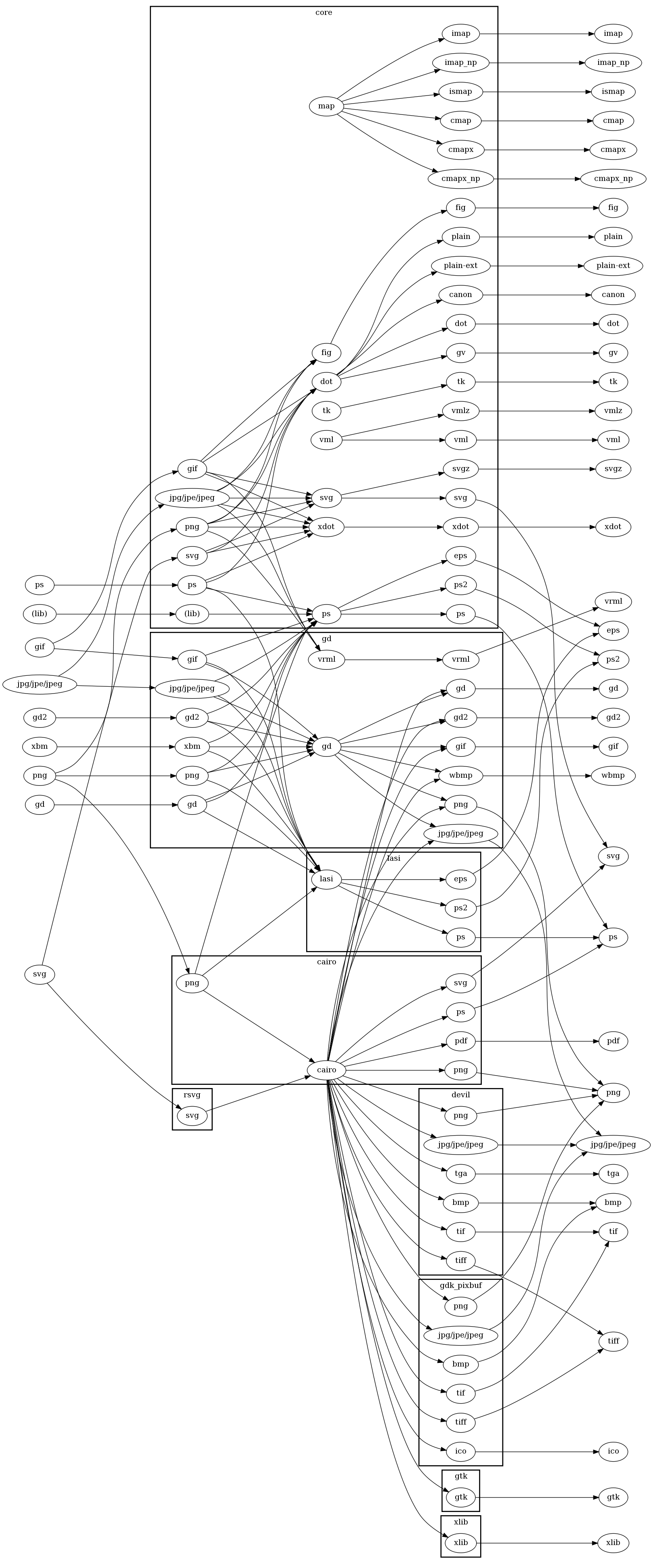
The graph below shows what image formats can be used in which output formats, and the required plugins. On the left are the supported image formats. On the right are the supported output formats. In the middle are the plugins: image loaders, renderers, drivers, arranged by plugin library. This presents the most general case. A given installation may not provide one of the plugins, in which case, that transformation is not possible.

ID Output Note

In the formats: -Tcmap, -Tcmapx, -Tsvg, -Tvml, the output generates id="node#" properties for nodes, id="edge#" properties for edges, and id="cluster#" properties for clusters, with the # replaced by an internally assigned integer. These strings can be provided instead by an externally provided id=xxx attribute on the object. Normal \N \E \G substitutions are applied. Externally provided id values are not used internally, and it is the user's reponsibilty to ensure that they are sufficiently unique for their intended downstream use. Note, in particular, that \E is not a unique id for multiedges.

4.1 - BMP

Windows Bitmap

Outputs images in the Windows BMP format.

4.2 - CGImage

Apple Core Graphics

Output using the Apple's Core Graphics Image format.

4.3 - DOT

Graphviz Language

These formats produce output in the dot language.

canon

Using canon produces a pretty printed version of the input, with no layout performed.

Example: simple graph, canonicalized formatting with -Tcanon


$ echo 'digraph { a->b }' | dot -Tcanon
digraph {
        node [label="\N"];
        a -> b;
}

dot / gv

The dot (and gv alias) options correspond to attributed dot output, and is the default output format. It reproduces the input, along with layout information for the graph. In particular, a bb attribute is attached to the graph, specifying the bounding box of the drawing. If the graph has a label, its position is specified by the lp attribute.

Each node gets pos, width and the record rectangles are given in the rects attribute. If the node is a polygon and the vertices attribute is defined, this attribute contains the vertices of the node.

Every edge is assigned a pos attribute, and if the edge has a label, the label position is given in lp.

Example: simple graph, outputting layout positioning with -Tdot


$ echo 'digraph { a->b }' | dot -Tdot
digraph {
        graph [bb="0,0,54,108"];
        node [label="\N"];
        a    [height=0.5,
             pos="27,90",
             width=0.75];
        b    [height=0.5,
             pos="27,18",
             width=0.75];
        a -> b  [pos="e,27,36.104 27,71.697 27,63.983 27,54.712 27,46.112"];
}

xdot

The xdot format extends the dot format by providing much more detailed information about how graph components are drawn. It relies on additional attributes for nodes, edges and graphs.

Attribute	Description	Limitations
`draw`	General drawing without labels
`ldraw`	Label drawing
`hdraw`	Head arrowhead	Edge only
`tdraw`	Tail arrowhead	Edge only
`hldraw`	Head label	Edge only
`tldraw`	Tail label	Edge only

Flag	Value	Min-Version
`BOLD`	1
`ITALIC`	2
`UNDERLINE`	4
`SUPERSCRIPT`	8
`SUBSCRIPT`	16	(1.5)
`STRIKE_THROUGH`	32	(1.6)
`OVERLINE`	64	(1.7)

Xdot version	Graphviz version	Modification
>1.0	1.9
>1.1	2.8	First plug-in version
>1.2	2.13	Support image operator I
>1.3	2.31	Add numerical precision
>1.4	2.32	Add gradient colors
>1.5	2.34	Fix text layout problem; fix inverted vector in gradient; support version-specific output; new t op for text characteristics
>1.6	2.35	Add STRIKE-THROUGH bit for`t`
>1.7	2.37	Add OVERLINE for `t`

4.4 - EPS

Encapsulated PostScript

Produces Encapsulated PostScript output.

At present, this is only guaranteed to be correct for a single input graph since the Bounding Box information has to appear at the beginning of the output, and this will be based on the first graph.

4.5 - EXR

OpenEXR

Output in the OpenEXR format

4.6 - FIG

Xfig

Outputs graphs in the FIG graphics language.

Example outputs of a simple graph with two nodes connected with an edge:


$ echo 'digraph { a->b }' | dot -Tfig
#FIG 3.2
# Generated by graphviz version 2.47.1 (20210417.1919)
# Title: %3
# Pages: 1
Portrait
Center
Inches
Letter
100.00
Single
-2
1200 2
0 32 #d3d3d3
0 33 #fffffe
2 3 0 1 33 7 2 0 20 0.0 0 0 0 0 0 5
 0 2320 0 0 1240 0 1240 2320 0 2320
# a
1 1 0 1 0 7 1 0 -1 0.000 0 0.0000 620 440 540 -360 620 440 1160 80
4 1 0 1 0 0 14.0 0.0000 6 14.0 4.7 620 498 a\001
# b
1 1 0 1 0 7 1 0 -1 0.000 0 0.0000 620 1880 540 -360 620 1880 1160 1520
4 1 0 1 0 0 14.0 0.0000 6 14.0 4.7 620 1938 b\001
# a->b
3 4 0 1 0 0 0 0 -1 0.0 0 0 0 7
  620 806 620 886 620 969 620 1055 620 1143 620 1231 620 1318
 0 1 1 1 1 1 0
2 3 0 1 0 0 0 0 20 0.0 0 0 0 0 0 4
 690 1318 620 1518 550 1318 690 1318
# end of FIG file

4.7 - GD/GD2

LibGD

Output images in the GD and GD2 format. These are the internal formats used by the gd library. gd2 is compressed.

4.8 - GIF

Graphics Interchange Format

Outputs images in GIF format.

4.9 - GTK

Formerly GTK+ / GIMP ToolKit

Creates a GTK window and displays the output there.

4.10 - ICO

Windows Icon

Outputs images in the Windows ICO format.

4.11 - Imagemap

Image Map: Server-side and client-side

imap and cmapx produce map files for server-side and client-side image maps. These can be used in a web page with a graphical form of the output, e.g. in JPEG, GIF or PNG format, to attach links to nodes and edges. Graphviz generates an object's map information only if the object has a non-trival URL or href attribute, or if it has an explicit tooltip attribute.

cmap produces map files for client-side image maps. It's mostly identical to cmapx, but the latter is well-formed XML amenable to processing by XML tools. In particular, the cmapx output is wrapped in <map></map>.

imap_np and cmapx_np are identical to the imap and cmapx formats, except they rely solely on rectangles as active areas.

ismap is a predecessor (circa 1994) of the imap format. Most servers now use the latter.

For example, to create a server-side map given the dot file:

/* x.gv */
digraph mainmap {
  URL="http://www.research.att.com/base.html";
  command [URL="http://www.research.att.com/command.html"];
  command -> output [URL="colors.html"];
}

Edit in Playground

one would process the graph and generate two output files:

dot -Timap -ox.map -Tgif -ox.gif x.gv

and then refer to it in a web page:

<A HREF="x.map"><IMG SRC="x.gif" ismap="ismap" /></A>

For client-side maps, one again generates two output files:

dot -Tcmapx -ox.map -Tgif -ox.gif x.gv

and uses the HTML

<IMG SRC="x.gif" USEMAP="#mainmap" />
... [content of x.map] ...

Note that the name given in the USEMAP attribute must be the same as the ID attribute of the MAP element. The Graphviz renderer uses the name of the graph as the ID. Thus, in the example above, where the graph's name is mainmap, we have USEMAP="#mainmap" in the IMG attribute, and x.map will look like

<map id="mainmap" name="mainmap">
... 
</map>

URLs can be attached to the root graph, nodes and edges. If a node has a URL, clicking in the node will activate the link. If an edge has a URL, various points along the edge (but not necessarily the head or tail) will link to it. In addition, if the edge has a label, that will link to the URL. As for the head of the edge, this is linked to the headURL, if set. Otherwise, it is linked to the edge's URL if that is defined. The analogous description holds for the tail and the tailURL. A URL associated with the graph is used as a default link.

If the URL of a node contains the escape sequence \N, it will be replaced by the node's name. If the headURL is defined and contains the escape sequence \N, it will be replaced by the headlabel, if defined. The analogous result holds for the tailURL and the taillabel.

See ID Output Note.

4.12 - JPEG

Joint Photographic Experts Group

Output JPEG-compressed image files.

JPEG's image compression can blur fine image details like text & lines, so consider using a lossless format (say, PNG or WebP) instead.

4.13 - JPEG 2000

Output using the JPEG 2000 format.

JPEG's image compression can blur fine image details like text & lines, so consider using a lossless format (say, PNG or WebP) instead.

4.14 - JSON

JavaScript Object Notation

These formats produce a JSON output encoding the DOT language.

json0 produces output in JSON format that contains the same information produced by -Tdot.
json produces output in JSON format that contains the same information produced by -Txdot.

Both of these assume the graph has been processed by one of the layout algorithms.

dot_json and xdot_json also produce JSON output similar to to json0 and json, respectively, except they only use the content of the graph on input. In particular, they do not assume that the graph has been processed by any layout algorithm, and the only xdot information appearing in the output was in the original input file.

The output produced by these follows the json schema shown below. Note that the objects array has all of the subgraphs first, followed by all of the nodes. The _gvid value is the index of the subgraph or node in the objects array. This also holds true for the edges in the objects array. Note that this format allows clustered graphs, where edges can connect clusters as well as nodes.

Example: simple graph rendered with -Tdot_json


$ echo 'digraph { a->b }' | dot -Tdot_json
{
  "name": "%3",
  "directed": true,
  "strict": false,
  "_subgraph_cnt": 0,
  "objects": [
    {
      "_gvid": 0,
      "name": "a",
      "label": "\\N"
    },
    {
      "_gvid": 1,
      "name": "b",
      "label": "\\N"
    }
  ],
  "edges": [
    {
      "_gvid": 0,
      "tail": 0,
      "head": 1
    }
  ]
}

Example: simple graph rendered with -Txdot_json


$ echo 'digraph { a->b }' | dot -Txdot_json
{
  "name": "%3",
  "directed": true,
  "strict": false,
  "_subgraph_cnt": 0,
  "objects": [
    {
      "_gvid": 0,
      "name": "a",
      "label": "\\N"
    },
    {
      "_gvid": 1,
      "name": "b",
      "label": "\\N"
    }
  ],
  "edges": [
    {
      "_gvid": 0,
      "tail": 0,
      "head": 1
    }
  ]
}

Example: simple graph rendered with -Tjson0


$ echo 'digraph { a->b }' | dot -Tjson0
{
  "name": "%3",
  "directed": true,
  "strict": false,
  "bb": "0,0,54,108",
  "_subgraph_cnt": 0,
  "objects": [
    {
      "_gvid": 0,
      "name": "a",
      "height": "0.5",
      "label": "\\N",
      "pos": "27,90",
      "width": "0.75"
    },
    {
      "_gvid": 1,
      "name": "b",
      "height": "0.5",
      "label": "\\N",
      "pos": "27,18",
      "width": "0.75"
    }
  ],
  "edges": [
    {
      "_gvid": 0,
      "tail": 0,
      "head": 1,
      "pos": "e,27,36.104 27,71.697 27,63.983 27,54.712 27,46.112"
    }
  ]
}

Example: simple graph rendered with -Tjson


echo 'digraph { a->b }' | dot -Tjson
{
  "name": "%3",
  "directed": true,
  "strict": false,
  "_draw_": 
  [
    {
      "op": "c",
      "grad": "none",
      "color": "#fffffe00"
    },
    {
      "op": "C",
      "grad": "none",
      "color": "#ffffff"
    },
    {
      "op": "P",
      "points": [[0.000,0.000],[0.000,108.000],[54.000,108.000],[54.000,0.000]]
    }
  ],
  "bb": "0,0,54,108",
  "xdotversion": "1.7",
  "_subgraph_cnt": 0,
  "objects": [
    {
      "_gvid": 0,
      "name": "a",
      "_draw_": 
      [
        {
          "op": "c",
          "grad": "none",
          "color": "#000000"
        },
        {
          "op": "e",
          "rect": [27.000,90.000,27.000,18.000]
        }
      ],
      "_ldraw_": 
      [
        {
          "op": "F",
          "size": 14.000,
          "face": "Times-Roman"
        },
        {
          "op": "c",
          "grad": "none",
          "color": "#000000"
        },
        {
          "op": "T",
          "pt": [27.000,86.300],
          "align": "c",
          "width": 7.000,
          "text": "a"
        }
      ],
      "height": "0.5",
      "label": "\\N",
      "pos": "27,90",
      "width": "0.75"
    },
    {
      "_gvid": 1,
      "name": "b",
      "_draw_": 
      [
        {
          "op": "c",
          "grad": "none",
          "color": "#000000"
        },
        {
          "op": "e",
          "rect": [27.000,18.000,27.000,18.000]
        }
      ],
      "_ldraw_": 
      [
        {
          "op": "F",
          "size": 14.000,
          "face": "Times-Roman"
        },
        {
          "op": "c",
          "grad": "none",
          "color": "#000000"
        },
        {
          "op": "T",
          "pt": [27.000,14.300],
          "align": "c",
          "width": 7.000,
          "text": "b"
        }
      ],
      "height": "0.5",
      "label": "\\N",
      "pos": "27,18",
      "width": "0.75"
    }
  ],
  "edges": [
    {
      "_gvid": 0,
      "tail": 0,
      "head": 1,
      "_draw_": 
      [
        {
          "op": "c",
          "grad": "none",
          "color": "#000000"
        },
        {
          "op": "b",
          "points": [[27.000,71.700],[27.000,63.980],[27.000,54.710],[27.000,46.110]]
        }
      ],
      "_hdraw_": 
      [
        {
          "op": "S",
          "style": "solid"
        },
        {
          "op": "c",
          "grad": "none",
          "color": "#000000"
        },
        {
          "op": "C",
          "grad": "none",
          "color": "#000000"
        },
        {
          "op": "P",
          "points": [[30.500,46.100],[27.000,36.100],[23.500,46.100]]
        }
      ],
      "pos": "e,27,36.104 27,71.697 27,63.983 27,54.712 27,46.112"
    }
  ]
}

description

JSON representation of a graph encoding xdot attributes

title

Graphviz JSON

required

name
directed
strict
_subgraph_cnt

definitions

drawops

items

oneOf

$ref
#/definitions/ellipse
#/definitions/polygon
#/definitions/polyline
#/definitions/bspline
#/definitions/text
#/definitions/font_style
#/definitions/drawcolor
#/definitions/font
#/definitions/style

type

array

style

required

op
style

type

object

properties

style

type	string

op

pattern	S
type	string

font_style

required

op
fontchar

type

object

properties

op

pattern	t
type	string

fontchar

minimum	0
type	integer
maximum	127

polygon

required

op
points

type

object

properties

points

$ref	#/definitions/pointlist

op

pattern	[pP]
type	string

metanode

required

_gvid
name

type

object

properties

_draw_

$ref	#/definitions/drawops

name

type	string
description	The node or subgraph name

_ldraw_

$ref	#/definitions/drawops

_gvid

type	integer

subgraphs

items

type	integer

type

array

description

index of a child subgraph

edges

items

type	integer

type

array

description

index of an edge in this subgraph

additionalProperties

type	string

nodes

items

type	integer

type

array

description

index of a node in this subgraph

title

node or subgraph

color

pattern	(#[0-9a-f]*)\|(#[0-9a-f]{8})
type	string

text

required

op
pt
align
text
width

type

object

properties

text

type	string

align

pattern	[lcr]
type	string

op

pattern	T
type	string

pt

$ref	#/definitions/point

width

type	number

point

minItems

2

items

type	number

type

array

maxItems

2

stop

required

frac
color

type

object

properties

color

$ref	#/definitions/color

frac

type	number

drawcolor

required

op
grad

type

object

properties

p0

oneOf

$ref
#/definitions/point
#/definitions/point3

p1

oneOf

$ref
#/definitions/point
#/definitions/point3

color

$ref	#/definitions/color

stops

items

$ref	#/definitions/stop

type

array

grad

enum	none linear radial
type	string

op

pattern	[cC]
type	string

ellipse

required

op
rect

type

object

properties

rect

$ref	#/definitions/rectangle

op

pattern	[eE]
type	string

bspline

required

op
points

type

object

properties

points

$ref	#/definitions/pointlist

op

pattern	[bB]
type	string

edge

required

_gvid
tail
head

type

object

properties

_hldraw_

$ref	#/definitions/drawops

_tdraw_

$ref	#/definitions/drawops

_draw_

$ref	#/definitions/drawops

_ldraw_

$ref	#/definitions/drawops

_gvid

type	integer

tail

type	integer
description	_gvid of tail node

_tldraw_

$ref	#/definitions/drawops

_hdraw_

$ref	#/definitions/drawops

additionalProperties

type	string

head

type	integer
description	_gvid of tail head

title

edge

polyline

required

op
points

type

object

properties

points

$ref	#/definitions/pointlist

op

pattern	L
type	string

font

required

op
size
face

type

object

properties

size

minimum	0
type	number

op

pattern	F
type	string

face

type	string

point3

minItems

3

items

type	number

type

array

maxItems

3

rectangle

minItems

4

items

type	number

type

array

maxItems

4

pointlist

items

$ref	#/definitions/point

type

array

type

object

properties

directed

type	boolean
description	True if the graph is directed

_draw_

$ref	#/definitions/drawops

name

type	string
description	The graph name

objects

items

$ref	#/definitions/metanode

type

array

description

The graph's subgraphs followed by the graph's nodes

_ldraw_

$ref	#/definitions/drawops

strict

type	boolean
description	True if the graph is strict

edges

items

$ref	#/definitions/edge

type

array

additionalProperties

type	string

_subgraph_cnt

type	integer
description	Number of subgraphs in the graph

4.15 - PDF

Portable Document Format

Produces PDF output. (This option assumes Graphviz includes the Cairo renderer.) Alternatively, one can use the ps2 option to produce PDF-compatible PostScript, and then use a ps-to-pdf converter.

4.16 - PIC

Brian Kernighan's Diagram Language

Output is given in the text-based PIC language developed for troff. See PIC language.

Example outputs of a simple graph with two nodes connected with an edge:


$ echo 'digraph { a->b }' | dot -Tpic
#  Creator: graphviz version 2.47.1 (20210417.1919)
#  Title: %3
#  save point size and font
.nr .S \n(.s
.nr DF \n(.f
.PS 0.86111 1.61111
#  to change drawing size, multiply the width and height on the .PS line above and the number on the two lines below (rounded to the nearest integer) by a scale factor
.nr SF 861
scalethickness = 861
#  don't change anything below this line in this drawing
#  non-fatal run-time pic version determination, version 2
boxrad=2.0 #  will be reset to 0.0 by gpic only
scale=1.0 #  required for comparisons
#  boxrad is now 0.0 in gpic, else it remains 2.0
#  dashwid is 0.1 in 10th Edition, 0.05 in DWB 2 and in gpic
#  fillval is 0.3 in 10th Edition (fill 0 means black), 0.5 in gpic (fill 0 means white), undefined in DWB 2
#  fill has no meaning in DWB 2, gpic can use fill or filled, 10th Edition uses fill only
#  DWB 2 doesn't use fill and doesn't define fillval
#  reset works in gpic and 10th edition, but isn't defined in DWB 2
#  DWB 2 compatibility definitions
if boxrad > 1.0 && dashwid < 0.075 then X
        fillval = 1;
        define fill Y Y;
        define solid Y Y;
        define reset Y scale=1.0 Y;
X
reset #  set to known state
#  GNU pic vs. 10th Edition d\(e'tente
if fillval > 0.4 then X
        define setfillval Y fillval = 1 - Y;
        define bold Y thickness 2 Y;
        #  if you use gpic and it barfs on encountering "solid",
        #       install a more recent version of gpic or switch to DWB or 10th Edition pic;
        #       sorry, the groff folks changed gpic; send any complaint to them;
X else Z
        define setfillval Y fillval = Y;
        define bold Y Y;
        define filled Y fill Y;
Z
#  arrowhead has no meaning in DWB 2, arrowhead = 7 makes filled arrowheads in gpic and in 10th Edition
#  arrowhead is undefined in DWB 2, initially 1 in gpic, 2 in 10th Edition
arrowhead = 7 #  not used by graphviz
#  GNU pic supports a boxrad variable to draw boxes with rounded corners; DWB and 10th Ed. do not
boxrad = 0 #  no rounded corners in graphviz
#  GNU pic supports a linethick variable to set line thickness; DWB and 10th Ed. do not
linethick = 0; oldlinethick = linethick
#  .PS w/o args causes GNU pic to scale drawing to fit 8.5x11 paper; DWB does not
#  maxpsht and maxpswid have no meaning in DWB 2.0, set page boundaries in gpic and in 10th Edition
#  maxpsht and maxpswid are predefined to 11.0 and 8.5 in gpic
maxpsht = 1.611111
maxpswid = 0.861111
Dot: [
define attrs0 % %; define unfilled % %; define rounded % %; define diagonals % %
move to (0, 0); line to (0, 116); line to (62, 116); line to (62, 0); line to (0, 0)
#  a
ellipse attrs0 wid 0.75000 ht 0.50000 at (0.43056,1.30556);
.ft R 
.ps 14*\n(SFu/861u
"a" at (27.54861,87.56481);
#  b
ellipse attrs0 wid 0.75000 ht 0.50000 at (0.43056,0.30556);
"b" at (27.54861,15.56481);
#  a->b
move to (31, 76); spline to (31, 72); spline to (31, 68); spline to (31, 63); spline to (31, 59); spline to (31, 54); spline to (31, 50)
move to (35, 50); line to (31, 40); line to (28, 50); line to (35, 50)
]
.PE
#  restore point size and font
.ps \n(.S
.ft \n(DF

4.17 - PICT

Apple PICT

Output in the Apple PICT file format.

4.18 - Plain Text

Simple, line-based language

The plain and plain-ext formats produce output using a simple, line-based language. The latter format differs in that, on edges, it provides port names on head and tail nodes when applicable.

Example outputs of a simple graph with two nodes connected with an edge:

-Tplain


$ echo 'digraph { a->b }' | dot -Tplain
graph 1 0.75 1.5
node a 0.375 1.25 0.75 0.5 a solid ellipse black lightgrey
node b 0.375 0.25 0.75 0.5 b solid ellipse black lightgrey
edge a b 4 0.375 0.99579 0.375 0.88865 0.375 0.7599 0.375 0.64045 solid black
stop

-Tplain-ext


$ echo 'digraph { a->b }' | dot -Tplain-ext
graph 1 0.75 1.5
node a 0.375 1.25 0.75 0.5 a solid ellipse black lightgrey
node b 0.375 0.25 0.75 0.5 b solid ellipse black lightgrey
edge a b 4 0.375 0.99579 0.375 0.88865 0.375 0.7599 0.375 0.64045 solid black
stop

There are four types of statements.

 graph scale width height
 node name x y width height label style shape color fillcolor
 edge tail head n x₁ y₁ .. xₙ yₙ [label xl yl] style color
 stop

graph

The width and height values give the width and height of the drawing. The lower left corner of the drawing is at the origin. The scale value indicates how the drawing should be scaled if a size attribute was given and the drawing needs to be scaled to conform to that size. If no scaling is necessary, it will be set to 1.0. Note that all graph, node and edge coordinates and lengths are given unscaled.

node

The name value is the name of the node, and x and y give the node's position. The width and height are the width and height of the node. The label, style, shape, color and fillcolor give the node's label, style, shape, color and fillcolor, respectively, using attribute default values where necessary. If the node does not have a style attribute, "solid" is used.

edge

The tail and head values give the names of the head and tail nodes. In plain-ext format, the head or tail name will be appended with a colon and a portname if the edge connects to the node at a port. n is the number of control points defining the B-spline forming the edge. This is followed by 2*n numbers giving the x and y coordinates of the control points in order from tail to head. If the edge has a label, this comes next followed by the x and y coordinates of the label's position. The edge description is completed by the edge's style and color. As with nodes, if a style is not defined, "solid" is used.

Note: The control points given in an edge statement define the body of the edge. In particular, if the edge has an arrowhead to the head or tail node, there will be a gap between the last or first control points and the boundary of the associated node. There are at least 3 possible ways of handling this gap:

Arrange that the input graph uses dir=none, arrowhead=none, or arrowtail=none for all edges. In this case, the terminating control points will always touch the node.
Consider the line segment joining the control point and the center of the node, and determine the point where the segment intersects the node's boundary. Then use the control point and the intersection point as the main axis of an arrowhead. The problem with this approach is that, if the edge has a port, the edge will not be pointing to the center of the node. In this case, rather than use the control point and center point, one can use the control point and its tangent.
Arrange that the input graph uses headclip=false or tailclip=false. In this case, the edge will terminate at the node's center rather than its boundary. If arrowheads are used, there will still be a gap, but normally this will occur within the node. The application will still need to clip the spline to the node boundary. Also, as with the previous item, if the edge points to a node port, this technique will fail.

The output consists of one graph line, a sequence of node lines, one per node, a sequence of edge lines, one per edge, and a final stop line. All units are in inches, represented by a floating point number.

Note that the plain formats provide minimal information, really giving not much more than node positions and sizes, and edge spline control points. These formats are usually most useful to applications wanting just this geometric information, and willing to fill in all of the graphical details. The only real advantages to these formats is their terseness and their ease of parsing. In general, the dot and xdot are preferable in terms of the quantity of information provided.

4.19 - PNG

Portable Network Graphics

Produces output in the PNG (Portable Network Graphics) format.

(25 November 2014) A standard Graphviz installation will render using both the Cairo and GD library. By mixing the rendering and formatting of these libraries, one can achieve different variations in the output.

-Tpng:gd (or -Tpng:gd:gd): Indexed color, no antialiasing
-Tpng:cairo:gd: Indexed color, with antialiasing
-Tpng (or -Tpng:cairo): True color, with antialiasing

These options are listed in increasing order of image quality and output size.

4.20 - POV-Ray

Persistence of Vision Raytracer (prototype)

Scene-description language for 3D modelling for the Persistence of Vision Raytracer.

Example: simple graph, rendered with -Tpov


$ echo 'digraph { a->b }' | dot -Tpov
#version 3.6;
global_settings { assumed_gamma 1.0 }
#default { finish { ambient 0.1 diffuse 0.9 } }
#include "colors.inc"
#include "textures.inc"
#include "shapes.inc"
#declare black = Black;
#declare white = White;
//*** begin_graph %3
camera { location <31.000 , 58.000 , -500.000>
         look_at  <31.000 , 58.000 , 0.000>
         right x * image_width / image_height
         angle 15.880
}
//sky
plane { <0, 1, 0>, 1 hollow
    texture {
        pigment { bozo turbulence 0.95
            color_map {
                [0.00 rgb <0.05, 0.20, 0.50>]
                [0.50 rgb <0.05, 0.20, 0.50>]
                [0.75 rgb <1.00, 1.00, 1.00>]
                [0.75 rgb <0.25, 0.25, 0.25>]
                [1.00 rgb <0.50, 0.50, 0.50>]
            }
            scale <1.00, 1.00, 1.50> * 2.50
            translate <0.00, 0.00, 0.00>
        }
        finish { ambient 1 diffuse 0 }
    }
    scale 10000
}
//mist
fog { fog_type 2
    distance 50
    color rgb <1.00, 1.00, 1.00> * 0.75
    fog_offset 0.10
    fog_alt 1.50
    turbulence 1.75
}
//gnd
plane { <0.00, 1.00, 0.00>, 0
    texture {
        pigment{ color rgb <0.25, 0.45, 0.00> }
        normal { bumps 0.75 scale 0.01 }
        finish { phong 0.10 }
    }
}
light_source { <1500,3000,-2500> color White }
//*** begin_page
//*** comment: a
//*** begin_node: a
//*** ellipse
torus { 1.000, 0.056
    scale    <   27.000,    11.250,    18.000>
    rotate   <   90.000,     0.000,     0.000>
    translate<   31.000,    94.000,    -6.000>
    pigment { color black transmit 0.000 }
}
//*** textspan: a, fontsize = 14.000, fontname = Times-Roman
text {
    ttf "Times-Roman",
    "a", 0.250, 0.000
        no_shadow
    scale 14.000
    rotate   <    0.000,     0.000,     0.000>
    translate<   27.500,    87.500,    -9.000>
    pigment { color black transmit 0.000 }
}
//*** end_node
//*** comment: b
//*** begin_node: b
//*** ellipse
torus { 1.000, 0.056
    scale    <   27.000,    11.250,    18.000>
    rotate   <   90.000,     0.000,     0.000>
    translate<   31.000,    22.000,    -6.000>
    pigment { color black transmit 0.000 }
}
//*** textspan: b, fontsize = 14.000, fontname = Times-Roman
text {
    ttf "Times-Roman",
    "b", 0.250, 0.000
        no_shadow
    scale 14.000
    rotate   <    0.000,     0.000,     0.000>
    translate<   27.500,    15.500,    -9.000>
    pigment { color black transmit 0.000 }
}
//*** end_node
//*** comment: a->b
//*** begin_edge
//*** bezier
sphere_sweep {
    b_spline
    6,
    <   31.000,    75.697,     0.000>, 1.000
    <   31.000,    75.697,     0.000>, 1.000
    <   31.000,    67.983,     0.000>, 1.000
    <   31.000,    58.712,     0.000>, 1.000
    <   31.000,    50.112,     0.000>, 1.000
    <   31.000,    50.112,     0.000>, 1.000
        tolerance 0.01
    scale    <    1.000,     1.000,     1.000>
    rotate   <    0.000,     0.000,     0.000>
    translate<    0.000,     0.000,   -11.000>
    pigment { color black transmit 0.000 }
}
//*** polygon
sphere_sweep {
    linear_spline
    4,
    <   34.500,    50.104,     0.000>, 1.000
    <   31.000,    40.104,     0.000>, 1.000
    <   27.500,    50.104,     0.000>, 1.000
    <   34.500,    50.104,     0.000>, 1.000
    tolerance 0.1
    scale    <    1.000,     1.000,     1.000>
    rotate   <    0.000,     0.000,     0.000>
    translate<    0.000,     0.000,    -9.000>
    pigment { color black transmit 0.000 }
}
polygon { 3,

    <   34.500,    50.104,     0.000>
    <   31.000,    40.104,     0.000>
    <   27.500,    50.104,     0.000>
    scale    <    1.000,     1.000,     1.000>
    rotate   <    0.000,     0.000,     0.000>
    translate<    0.000,     0.000,    -9.000>
    pigment { color black transmit 0.250 }
}
//*** end_edge
//*** end_page
//*** end_graph

4.21 - PS

Adobe PostScript

Produces Adobe PostScript format output.

Note: The default PostScript renderer can only handle the Latin-1 character set. To get non-Latin-1 characters into PostScript output, use -Tps:cairo, assuming your version was built with the Cairo renderer.

4.22 - PS/PDF

Adobe PostScript for Portable Document Format

Produces PostScript output with PDF notations.

It is assumed the output will be directly converted into PDF format. The notations include PDF bounding box information, so that the resulting PDF file can be correctly used with pdf tools, such as pdflatex. In addition, if a node has a URL attribute, this gets translated into PDF code such that the node, when viewed in a PDF-viewer, e.g., Adobe Acrobat, is a link to the given URL. If a URL is attached to the graph, this serves as a base, such that relative URLs on nodes are derived from it.

4.23 - PSD

Photoshop

Output in the Adobe PhotoShop PSD file format.

4.24 - SGI

Silicon Graphics Image

Output in the SGI (Silicon Graphics Image) file format.

4.25 - SVG

Scalable Vector Graphics

svg produces SVG output.

svgz produces compressed SVGs.

See ID Output Note.

Example: simple graph rendered with -Tsvg


$ echo 'digraph { a->b }' | dot -Tsvg
<?xml version="1.0" encoding="UTF-8" standalone="no"?>
<!DOCTYPE svg PUBLIC "-//W3C//DTD SVG 1.1//EN"
 "http://www.w3.org/Graphics/SVG/1.1/DTD/svg11.dtd">
<!-- Generated by graphviz version 2.47.1 (20210417.1919)
 -->
<!-- Pages: 1 -->
<svg width="62pt" height="116pt"
 viewBox="0.00 0.00 62.00 116.00" xmlns="http://www.w3.org/2000/svg" xmlns:xlink="http://www.w3.org/1999/xlink">
<g id="graph0" class="graph" transform="scale(1 1) rotate(0) translate(4 112)">
<polygon fill="white" stroke="transparent" points="-4,4 -4,-112 58,-112 58,4 -4,4"/>
<!-- a -->
<g id="node1" class="node">
<title>a</title>
<ellipse fill="none" stroke="black" cx="27" cy="-90" rx="27" ry="18"/>
<text text-anchor="middle" x="27" y="-86.3" font-family="Times,serif" font-size="14.00">a</text>
</g>
<!-- b -->
<g id="node2" class="node">
<title>b</title>
<ellipse fill="none" stroke="black" cx="27" cy="-18" rx="27" ry="18"/>
<text text-anchor="middle" x="27" y="-14.3" font-family="Times,serif" font-size="14.00">b</text>
</g>
<!-- a&#45;&gt;b -->
<g id="edge1" class="edge">
<title>a&#45;&gt;b</title>
<path fill="none" stroke="black" d="M27,-71.7C27,-63.98 27,-54.71 27,-46.11"/>
<polygon fill="black" stroke="black" points="30.5,-46.1 27,-36.1 23.5,-46.1 30.5,-46.1"/>
</g>
</g>
</svg>

4.26 - TGA

Truevision TARGA

Output in the Truevision TGA or TARGA format.

4.27 - TIFF

Tag Image File Format

Produces TIFF output.

4.28 - Tk

Tcl/Tk

Output using the text-based Tcl/Tk graphics primitives.

Example outputs of a simple graph with two nodes connected with an edge:

Example: simple graph rendered with -Ttk


$ echo 'digraph { a->b }' | dot -Ttk
# Generated by graphviz version 2.47.1 (20210417.1919)
# Title: %3 Pages: 1
# a
$c create oval 5.3333 53.3333 77.3333 5.3333 -fill white -width 1 -outline black -tags {1node0x75509df0}
$c create text 41.3333 30.3 -text {a} -fill black -font {"Times" 14} -tags {0node0x75509df0}
# b
$c create oval 5.3333 149.3333 77.3333 101.3333 -fill white -width 1 -outline black -tags {1node0x75509f10}
$c create text 41.3333 126.3 -text {b} -fill black -font {"Times" 14} -tags {0node0x75509f10}
# a->b
$c create line 41.3333 53.7378 41.3333 64.023 41.3333 76.3834 41.3333 87.8501 -fill black -width 1 -smooth bezier  -tags {1edge0x5}
$c create polygon 46.0001 87.8609 41.3333 101.1942 36.6668 87.8608 -fill black -width 1 -outline black -tags {1edge0x5}

4.29 - VML

Vector Markup Language.

Deprecated: Removed in Graphviz 8.0.1.

Produces VML output, the latter in compressed format.

VML is obsolete, superseded by SVG.

See ID Output Note.

4.30 - VRML

Virtual Reality Modeling Language

Outputs graphs in the VRML format. To get a 3D embedding, nodes must have a z attribute. These can either be supplied as part of the input graph, or be generated by neato provided dim=3 and at least one node has a z value.

Line segments are drawn as cylinders. In general, VRML output relies on having the PNG library to produce images used to texture-fill the node shapes. However, if shape=point, a node is drawn as a 3D sphere.

Example: simple graph, rendered with -Tvrml


$ echo 'digraph { a->b }' | dot -Tvrml
#VRML V2.0 utf8
Group { children [
  Transform {
    scale 0.028 0.028 0.028
    children [
 Background { skyColor 1.000 1.000 1.000 }
# node a
Transform {
  translation 27.000 90.000 0.000
  scale 27.000 18.000 1
  children [
    Transform {
      rotation 1 0 0   1.57
      children [
        Shape {
          geometry Cylinder { side FALSE }
          appearance Appearance {
            material Material {
              ambientIntensity 0.33
              diffuseColor 1 1 1
            }
            texture ImageTexture { url "node1.png" }
          }
        }
      ]
    }
  ]
}
# node b
Transform {
  translation 27.000 18.000 0.000
  scale 27.000 18.000 1
  children [
    Transform {
      rotation 1 0 0   1.57
      children [
        Shape {
          geometry Cylinder { side FALSE }
          appearance Appearance {
            material Material {
              ambientIntensity 0.33
              diffuseColor 1 1 1
            }
            texture ImageTexture { url "node2.png" }
          }
        }
      ]
    }
  ]
}
# edge a -> b
 Group { children [
Transform {
  children [
    Shape {
      geometry Cylinder {
        bottom FALSE top FALSE
        height 25.584 radius 1.000 }
      appearance Appearance {
        material Material {
          ambientIntensity 0.33
          diffuseColor 0.000 0.000 0.000
        }
      }
    }
Transform {
  translation 0 17.792 0
  children [
    Shape {
      geometry Cone {bottomRadius 3.500 height 10.000 }
      appearance Appearance {
        material Material {
          ambientIntensity 0.33
          diffuseColor 0.000 0.000 0.000
        }
      }
    }
  ]
}
      ]
      center 0 5.000 0
      rotation -0.000 0 1.000 -3.142
      translation 27.000 49.000 0.000
    }
] }
  ] }
  Viewpoint {position 1.000 2.000 6.438}
] }

4.31 - WBMP

Wireless Bitmap

Produces output in the monochrome Wireless BitMap (WBMP) format, optimized for mobile computing.

4.32 - WebP

WebP

Produces output in the image format for the Web (WEBP) format, optimized for web devices such as tablets. See Wikipedia's WebP or Google's WebP pages.

4.33 - X11

X11 Window

Creates an Xlib (X11) window and displays the output there.

xlib is an alias for x11.

5 - Attributes

Instructions to customise the layout of Graphviz nodes, edges, graphs, subgraphs, and clusters.

The table below describes the attributes used by various Graphviz tools. The table gives the name of the attribute, the graph components (node, edge, etc.) which use the attribute and the type of the attribute (strings representing legal values of that type). Where applicable, the table also gives a default value for the attribute, a minimum allowed setting for numeric attributes, and certain restrictions on the use of the attribute.

Note that attribute names are case-sensitive. This is usually true for attribute values as well, unless noted.

All Graphviz attributes are specified by name-value pairs. Thus, to set the color of a node abc, one would use

digraph {
  abc [color = red]
}

Edit in Playground

Similarly, to set the arrowhead style of an edge abc -> def, one would use:

digraph {
  abc -> def [arrowhead = diamond]
}

Edit in Playground

Further details concerning the setting of attributes can be found in the description of the DOT language.

At present, most device-independent units are either inches or points, which we take as 72 points per inch.

Note: Some attributes, such as dir or arrowtail, are ambiguous when used in DOT with an undirected graph since the head and tail of an edge are meaningless. As a convention, the first time an undirected edge appears, the DOT parser will assign the left node as the tail node and the right node as the head. For example, the edge A -- B will have tail A and head B. It is the user's responsibility to handle such edges consistently. If the edge appears later, in the format

graph {
  B -- A [taillabel = "tail"]
}

Edit in Playground

the drawing will attach the tail label to node A. To avoid possible confusion when such attributes are required, the user is encouraged to use a directed graph. If it is important to make the graph appear undirected, this can be done using the dir, arrowtail or arrowhead attributes.

The tools accept standard C representations for int and double types. For the bool type, TRUE values are represented by true or yes (case-insensitive) and any non-zero integer, and FALSE values by false or no (case-insensitive) and zero. In addition, there are a variety of specialized types such as arrowType, color, point and rankdir. Legal values for these types are given at the end.

The Used By column field indicates which graph component(s) the attribute applies to.

In the Notes field, an annotation of write only indicates that the attribute is used for output, and is not used or read by any of the layout programs.

5.1 - _background

A string in the xdot format specifying an arbitrary background

During rendering, the canvas is first filled as described in the bgcolor attribute.

Then, if _background is defined, the graphics operations described in the string are performed on the canvas.

See xdot format page for more information.

Render a red square in the background

digraph G {
  _background="c 7 -#ff0000 p 4 4 4 36 4 36 36 4 36";
  a -> b
}

Edit in Playground

5.2 - area

Indicates the preferred area for a node or empty cluster

Example: Australian Coins, area proportional to value

graph {
  layout="patchwork"
  node [style=filled]
  "5c"  [area=  5 fillcolor=silver]
  "10c" [area= 10 fillcolor=silver]
  "20c" [area= 20 fillcolor=silver]
  "50c" [area= 50 fillcolor=silver]
  "$1"  [area=100 fillcolor=gold]
  "$2"  [area=200 fillcolor=gold]
}

Edit in Playground

5.3 - arrowhead

Style of arrowhead on the head node of an edge

This will only appear if the dir attribute is forward or both.

See the limitation.

See also:

arrowtail

5.4 - arrowsize

Multiplicative scale factor for arrowheads

Example

digraph {
  quiver -> "0.5" [arrowsize=0.5]
  quiver -> "1"
  quiver -> "2" [arrowsize=2]
  quiver -> "3" [arrowsize=3]
}

Edit in Playground

5.5 - arrowtail

Style of arrowhead on the tail node of an edge

This will only appear if the dir attribute is back or both.

See the limitation.

See also:

arrowhead

5.6 - bb

Bounding box of drawing in points

5.7 - beautify

Whether to draw leaf nodes uniformly in a circle around the root node in sfdp.

Whether to try to draw leaf nodes uniformly on a circle around the root node.

Prior to Graphviz 8.0.1, this is affected by Issue 2283: rendering one fewer sector than necessary, overlapping the first and last nodes.

Examples:

Beautify

digraph G {
    layout="sfdp"
    beautify=true

    N0 -> {N1; N2; N3; N4; N5; N6}
}

Edit in Playground

No beautify

digraph G {
    layout="sfdp"
    beautify=false

    N0 -> {N1; N2; N3; N4; N5; N6}
}

Edit in Playground

5.8 - bgcolor

Canvas background color

When attached to the root graph, this color is used as the background for entire canvas.

When a cluster attribute, it is used as the initial background for the cluster. If a cluster has a filled style, the cluster's fillcolor will overlay the background color.

If the value is a colorList, a gradient fill is used. By default, this is a linear fill; setting style=radial will cause a radial fill. Only two colors are used. If the second color (after a colon) is missing, the default color is used for it. See also the gradientangle attribute for setting the gradient angle.

For certain output formats, such as PostScript, no fill is done for the root graph unless bgcolor is explicitly set.

For bitmap formats, however, the bits need to be initialized to something, so the canvas is filled with white by default. This means that if the bitmap output is included in some other document, all of the bits within the bitmap's bounding box will be set, overwriting whatever color or graphics were already on the page. If this effect is not desired, and you only want to set bits explicitly assigned in drawing the graph, set bgcolor="transparent".

Example

graph {
  bgcolor="lightblue"
  label="Home"
  subgraph cluster_ground_floor {
    bgcolor="lightgreen"
    label="Ground Floor"
    Lounge
    Kitchen
  }
  subgraph cluster_top_floor {
    bgcolor="lightyellow"
    label="Top Floor"
    Bedroom
    Bathroom
  }
}

Edit in Playground

5.9 - center

Whether to center the drawing in the output canvas

Can be true or false.

5.10 - charset

Character encoding used when interpreting string input as a text label.

The default value is "UTF-8". The other legal values are:

"utf-8" / "utf8" (default value)
"iso-8859-1" / "ISO_8859-1" / "ISO8859-1" / "ISO-IR-100" / "Latin1" / "l1" / "latin-1"
"big-5" / "big5": the Big-5 Chinese encoding

The charset attribute is case-insensitive.

Note that if the character encoding used in the input does not match the charset value, the resulting output may be very strange.

Example

digraph G {
  charset="UTF-8"
  "🍔" -> "💩"
}

Edit in Playground

5.11 - class

Classnames to attach to the node, edge, graph, or cluster's SVG element

Combine with stylesheet for styling SVG output using CSS classnames.

Multiple space-separated classes are supported.

See also:

Example:

digraph G {
  graph [class="cats"];

  subgraph cluster_big {
    graph [class="big_cats"];

    "Lion" [class="yellow social"];
    "Snow Leopard" [class="white solitary"];
  }
}

Edit in Playground

5.12 - cluster

Whether the subgraph is a cluster

Subgraph clusters are rendered differently, e.g. dot renders a box around subgraph clusters, but doesn't draw a box around non-subgraph clusters.

Example:

digraph cats {
  subgraph cluster_big_cats {
    // This subgraph is a cluster, because the name begins with "cluster"
    
    "Lion";
    "Snow Leopard";
  }

  subgraph domestic_cats {
    // This subgraph is also a cluster, because cluster=true.
    cluster=true;

    "Siamese";
    "Persian";
  }

  subgraph not_a_cluster {
    // This subgraph is not a cluster, because it doesn't start with "cluster",
    // nor sets cluster=true.
    
    "Wildcat";
  }
}

Edit in Playground

5.13 - clusterrank

Mode used for handling clusters

If clusterrank=local, a subgraph whose name begins with cluster is given special treatment.

The subgraph is laid out separately, and then integrated as a unit into its parent graph, with a bounding rectangle drawn about it. If the cluster has a label parameter, this label is displayed within the rectangle.

Note also that there can be clusters within clusters.

The modes clusterrank=global and clusterrank=none appear to be identical, both turning off the special cluster processing.

5.14 - color

Basic drawing color for graphics, not text

For the latter, use the fontcolor attribute.

For edges, the value can either be a single color or a colorList.

In the latter case, if colorList has no fractions, the edge is drawn using parallel splines or lines, one for each color in the list, in the order given.

The head arrow, if any, is drawn using the first color in the list, and the tail arrow, if any, the second color. This supports the common case of drawing opposing edges, but using parallel splines instead of separately routed multiedges.

If any fraction is used, the colors are drawn in series, with each color being given roughly its specified fraction of the edge.

For example, the graph:

Edge Color Example

digraph G {
  a -> b [dir=both color="red:blue"]
  c -> d [dir=none color="green:red;0.25:blue"]
}

Edit in Playground

yields:

Subgraph & Node Color Example

digraph G {
  subgraph cluster_yellow {
    color="yellow"
    a [color="red"]
    b [color="green"]
  }
}

Edit in Playground

yields:

See also:

colorscheme

5.15 - colorscheme

A color scheme namespace: the context for interpreting color names

In particular, if a color value has form "xxx" or "//xxx", then the color xxx will be evaluated according to the current color scheme. If no color scheme is set, the standard X11 naming is used.

For example, if colorscheme=oranges9 (from Brewer color schemes), then color=7 is interpreted as color="/oranges9/7", the 7th color in the oranges9 colorscheme.

Orange Colorscheme

graph {
  node [colorscheme=oranges9] # Apply colorscheme to all nodes
  1 [color=1]
  2 [color=2]
  3 [color=3]
  4 [color=4]
  5 [color=5]
  6 [color=6]
  7 [color=7]
  8 [color=8]
  9 [color=9]
}

Edit in Playground

Green Colorscheme

graph {
  node [colorscheme=greens9] # Apply colorscheme to all nodes
  1 [color=1]
  2 [color=2]
  3 [color=3]
  4 [color=4]
  5 [color=5]
  6 [color=6]
  7 [color=7]
  8 [color=8]
  9 [color=9]
}

Edit in Playground

See also:

color

5.16 - comment

Comments are inserted into output

Device-dependent.

Example

digraph {
  comment="I am a graph"
  A [comment="I am node A"]
  B [comment="I am node B"]
  A->B [comment="I am an edge"]
}

Edit in Playground

Outputs SVG with comments:

<?xml version="1.0" encoding="UTF-8" standalone="no"?>
<!DOCTYPE svg PUBLIC "-//W3C//DTD SVG 1.1//EN"
 "http://www.w3.org/Graphics/SVG/1.1/DTD/svg11.dtd">
<!-- Generated by graphviz version 2.47.1 (20210417.1919)
 -->
<!-- This is a graph -->
<!-- Pages: 1 -->
<svg width="62pt" height="116pt"
 viewBox="0.00 0.00 62.00 116.00" xmlns="http://www.w3.org/2000/svg" xmlns:xlink="http://www.w3.org/1999/xlink">
<g id="graph0" class="graph" transform="scale(1 1) rotate(0) translate(4 112)">
<polygon fill="white" stroke="transparent" points="-4,4 -4,-112 58,-112 58,4 -4,4"/>
<!-- A -->
<!-- I am node A -->
<g id="node1" class="node">
<title>A</title>
<ellipse fill="none" stroke="black" cx="27" cy="-90" rx="27" ry="18"/>
<text text-anchor="middle" x="27" y="-86.3" font-family="Times,serif" font-size="14.00">A</text>
</g>
<!-- B -->
<!-- I am node B -->
<g id="node2" class="node">
<title>B</title>
<ellipse fill="none" stroke="black" cx="27" cy="-18" rx="27" ry="18"/>
<text text-anchor="middle" x="27" y="-14.3" font-family="Times,serif" font-size="14.00">B</text>
</g>
<!-- A&#45;&gt;B -->
<!-- I am an edge -->
<g id="edge1" class="edge">
<title>A&#45;&gt;B</title>
<path fill="none" stroke="black" d="M27,-71.7C27,-63.98 27,-54.71 27,-46.11"/>
<polygon fill="black" stroke="black" points="30.5,-46.1 27,-36.1 23.5,-46.1 30.5,-46.1"/>
</g>
</g>
</svg>

5.17 - compound

If true, allow edges between clusters

See lhead and ltail.

digraph {
  compound=true;

  subgraph cluster_a {
    label="Cluster A";
    node1; node3; node5; node7;
  }
  subgraph cluster_b {
    label="Cluster B";
    node2; node4; node6; node8;
  }

  node1 -> node2 [label="1"];
  node3 -> node4 [label="2" ltail="cluster_a"];
  
  node5 -> node6 [label="3" lhead="cluster_b"];
  node7 -> node8 [label="4" ltail="cluster_a" lhead="cluster_b"];
}

Edit in Playground

5.18 - concentrate

If true, use edge concentrators

This merges multiedges into a single edge and causes partially parallel edges to share part of their paths. The latter feature is not yet available outside of dot.

Example

digraph {
    concentrate=true
    a -> b [label="1"]
    c -> b
    d -> b
}

Edit in Playground

5.19 - constraint

If false, the edge is not used in ranking the nodes

For example in the graph:

digraph G {
  a -> c;
  a -> b;
  b -> c [constraint=false];
}

Edit in Playground

the edge b -> c does not add a constraint during rank assignment, so the only constraints are that a be above b and c, yielding the graph:

5.20 - Damping

Factor damping force motions.

On each iteration, a node's movement is limited to this factor of its potential motion. By being less than 1.0, the system tends to "cool", thereby preventing cycling.

5.21 - decorate

Whether to connect the edge label to the edge with a line

If true, attach edge label to edge by a 2-segment polyline, underlining the label, then going to the closest point of spline.

Example

digraph {
  a -> a [label="AA" decorate=true]
  a -> b [label="AB" decorate=true]
  b -> b [label="BB" decorate=false]
}

Edit in Playground

5.22 - defaultdist

The distance between nodes in separate connected components

If set too small, connected components may overlap.

Only applicable if pack=false.

5.23 - dim

Set the number of dimensions used for the layout

The maximum value allowed is 10.

5.24 - dimen

Set the number of dimensions used for rendering

The maximum value allowed is 10.

If both dimen and dim are set, the latter specifies the dimension used for layout, and the former for rendering. If only dimen is set, this is used for both layout and rendering dimensions.

Note that, at present, all aspects of rendering are 2D. This includes the shape and size of nodes, overlap removal, and edge routing. Thus, for dimen > 2, the only valid information is the pos attribute of the nodes.

All other coordinates will be 2D and, at best, will reflect a projection of a higher-dimensional point onto the plane.

5.25 - dir

Edge type for drawing arrowheads

Indicates which ends of the edge should be decorated with an arrowhead.

The actual style of the arrowhead can be specified using the arrowhead and arrowtail attributes.

See limitation.

Example

digraph {
  A->B [dir=forward]
  C->D [dir=back]
  E->F [dir=both]
  G->H [dir=none]
}

Edit in Playground

5.26 - diredgeconstraints

Whether to constrain most edges to point downwards

If true, constraints are generated for each edge in the largest (heuristic) directed acyclic subgraph such that the edge must point downwards.

Only valid when mode="ipsep".

If hier, generates level constraints similar to those used with mode="hier". The main difference is that, in the latter case, only these constraints are involved, so a faster solver can be used.

5.27 - distortion

Distortion factor for shape=polygon

Positive values cause top part to be larger than bottom; negative values do the opposite.

5.28 - dpi

Specifies the expected number of pixels per inch on a display device

For bitmap output, dpi guarantees that text rendering will be done more accurately, both in size and in placement.

For SVG output, dpi guarantees the dimensions in the output correspond to the correct number of points or inches.

5.29 - edgehref

Synonym for edgeURL

See also:

5.30 - edgetarget

Browser window to use for the edgeURL link

If the edge has a URL or edgeURL attribute, edgetarget determines which window of the browser is used for the URL attached to the non-label part of the edge.

Setting edgetarget=_graphviz will open a new window if it doesn't already exist, or reuse it if it does.

If undefined, the value of the target is used instead.

5.31 - edgetooltip

Tooltip annotation attached to the non-label part of an edge

5.32 - edgeURL

The link for the non-label parts of an edge

edgeURL overrides any URL defined for the edge.

Also, edgeURL is used near the head or tail node unless overridden by headURL or tailURL, respectively.

See limitation.

See also:

5.33 - epsilon

Terminating condition

If the length squared of all energy gradients are less than epsilon, the algorithm stops.

5.34 - esep

Margin used around polygons for purposes of spline edge routing

The interpretation is the same as given for sep. esep should normally be strictly less than sep.

5.35 - fillcolor

Color used to fill the background of a node or cluster

Assuming style=filled, or a filled arrowhead.

If fillcolor is not defined, color is used. (For clusters, if color is not defined, bgcolor is used.) If this is not defined, the default is used, except for shape=point or when the output format is MIF, which use black by default.

If the value is a colorList, a gradient fill is used. By default, this is a linear fill; setting style=radial will cause a radial fill. At present, only two colors are used. If the second color (after a colon) is missing, the default color is used for it.

See also the gradientangle attribute for setting the gradient angle.

Note that a cluster inherits the root graph's attributes if defined. Thus, if the root graph has defined a fillcolor, this will override a color or bgcolor attribute set for the cluster.

5.36 - fixedsize

Whether to use the specified width and height attributes to choose node size (rather than sizing to fit the node contents)

If false, the size of a node is determined by smallest width and height needed to contain its label and image, if any, with a margin specified by the margin attribute.

The width and height must also be at least as large as the sizes specified by the width and height attributes, which specify the minimum values for these parameters.

If true, the node size is specified by the values of the width and height attributes only and is not expanded to contain the text label. There will be a warning if the label (with margin) cannot fit within these limits.

If the fixedsize attribute is set to shape, the width and height attributes also determine the size of the node shape, but the label can be much larger. Both the label and shape sizes are used when avoiding node overlap, but all edges to the node ignore the label and only contact the node shape. No warning is given if the label is too large.

5.37 - fontcolor

Color used for text

5.38 - fontname

Font used for text

This very much depends on the output format and, for non-bitmap output such as PostScript or SVG, the availability of the font when the graph is displayed or printed. As such, it is best to rely on font faces that are generally available, such as Times-Roman, Helvetica or Courier.

How font names are resolved also depends on the underlying library that handles font name resolution. If Graphviz was built using the fontconfig library, the latter library will be used to search for the font. See the commands fc-list, fc-match and the other fontconfig commands for how names are resolved and which fonts are available. Other systems may provide their own font package, such as Quartz for OS X.

Note that various font attributes, such as weight and slant, can be built into the font name. Unfortunately, the syntax varies depending on which font system is dominant. Thus, using fontname="times bold italic" will produce a bold, slanted Times font using Pango, the usual main font library. Alternatively, fontname="times:italic" will produce a slanted Times font from fontconfig, while fontname="times-bold" will resolve to a bold Times using Quartz. You will need to ascertain which package is used by your Graphviz system and refer to the relevant documentation.

If Graphviz is not built with a high-level font library, fontname will be considered the name of a Type 1 or True Type font file. If you specify fontname=schlbk, the tool will look for a file named schlbk.ttf or schlbk.pfa or schlbk.pfb in one of the directories specified by the fontpath attribute. The lookup does support various aliases for the common fonts.

digraph {
    label="Comic Sans MS"
    fontname="Comic Sans MS"
    subgraph cluster_a {
      label="Courier New"
      fontname="Courier New"
      Arial [fontname="Arial"];
      Arial -> Arial [label="Impact" fontname="Impact"]
    }
}

Edit in Playground

5.39 - fontnames

Allows user control of how basic fontnames are represented in SVG output

If fontnames is undefined or svg, the output will try to use known SVG fontnames.

For example, the default font Times-Roman will be mapped to the basic SVG font serif. This can be overridden by setting fontnames to ps or hd. In the former case, known PostScript font names such as Times-Roman will be used in the output. In the latter case, the fontconfig font conventions are used. Thus, Times-Roman would be treated as Nimbus Roman No9 L. These last two options are useful with SVG viewers that support these richer fontname spaces.

5.40 - fontpath

Directory list used by libgd to search for bitmap fonts

Used if Graphviz was not built with the fontconfig library.

If fontpath is not set, the environment variable DOTFONTPATH is checked.

If DOTFONTPATH is not set, GDFONTPATH is checked.

If GDFONTPATH not set, libgd uses its compiled-in font path.

Note that fontpath is an attribute of the root graph.

5.41 - fontsize

Font size, in points, used for text

digraph {
    label="40pt Graph Label"
    fontsize="40"
    subgraph cluster_a {
      label="30pt Cluster Label"
      fontsize="30pt"
      "20pt Node" [fontsize="20pt"];
      "20pt Node"-> "20pt Node" [label="10pt Edge" fontsize="10"]
    }
}

Edit in Playground

5.42 - forcelabels

Whether to force placement of all xlabels, even if overlapping

If true, all xlabel attributes are placed, even if there is some overlap with nodes or other labels.

5.43 - gradientangle

If a gradient fill is being used, this determines the angle of the fill

For linear fills, the colors transform along a line specified by the angle and the center of the object. For radial fills, a value of zero causes the colors to transform radially from the center; for non-zero values, the colors transform from a point near the object's periphery as specified by the value.

If unset, the default angle is 0.

5.44 - group

Name for a group of nodes, for bundling edges avoiding crossings.

If the end points of an edge belong to the same group, i.e., have the same group attribute, parameters are set to avoid crossings and keep the edges straight.

5.45 - head_lp

Center position of an edge's head label

In points.

5.46 - headclip

If true, the head of an edge is clipped to the boundary of the head node

Otherwise, the end of the edge goes to the center of the node, or the center of a port, if applicable.

5.47 - headhref

Synonym for headURL

See also:

5.48 - headlabel

Text label to be placed near head of edge

See limitation.

5.49 - headport

Indicates where on the head node to attach the head of the edge

In the default case, the edge is aimed towards the center of the node, and then clipped at the node boundary.

See limitation.

5.50 - headtarget

Browser window to use for the headURL link

If the edge has a headURL, headtarget determines which window of the browser is used for the URL. Setting headURL=_graphviz will open a new window if the window doesn't already exist, or reuse the window if it does.

If undefined, the value of the target is used.

5.51 - headtooltip

Tooltip annotation attached to the head of an edge

Used only if the edge has a headURL attribute.

See also:

5.52 - headURL

If defined, headURL is output as part of the head label of the edge

Also, this value is used near the head node, overriding any URL value.

See limitation.

See also:

5.53 - height

Height of node, in inches

This is taken as the initial, minimum height of the node. If fixedsize is true, this will be the final height of the node. Otherwise, if the node label requires more height to fit, the node's height will be increased to contain the label.

If the output format is dot, the value given to height will be the final value.

If the node shape is regular, the width and height are made identical:

If both the width and the height are set explicitly, the maximum of the two values is used.
If one of width or height is set explicitly, that value is used for both width and height.
If neither is set explicitly, the minimum of the two default values is used.

Height Example

digraph G {
  "default"
  "1in" [height=1]
  "2in" [height=2]
}

Edit in Playground

See also:

width

5.54 - href

Synonym for URL

See also:

5.55 - id

Identifier for graph objects

Allows the graph author to provide an identifier for graph objects which is to be included in the output.

Normal \N, \E, \G substitutions are applied.

If provided, it is the responsibility of the provider to keep id values unique for its intended downstream use.

Note, in particular, that \E does not provide a unique id for multi-edges.

If no id attribute is provided, then a unique internal id is used. However, this value is unpredictable by the graph writer.

If the graph provides an id attribute, this will be used as a prefix for internally generated attributes. By making internally-used attributes distinct, the user can include multiple image maps in the same document.

5.56 - image

Gives the name of a file containing an image to be displayed inside a node

The image file must be in one of the recognized formats, typically JPEG, PNG, GIF, BMP, SVG, or Postscript, and be able to be converted into the desired output format.

The file must contain the image size information:

Bitmap formats usually already contain image size.
PostScript files must contain a line starting with %%BoundingBox: followed by four integers specifying the lower left x and y coordinates and the upper right x and y coordinates of the bounding box for the image, the coordinates being in points.
An SVG image file must contain width and height attributes, typically as part of the svg element. The values for these should have the form of a floating point number, followed by optional units, e.g., width="76pt". Recognized units are in, px, pc, pt, cm and mm for inches, pixels, picas, points, centimeters and millimeters, respectively. The default unit is points.

Unlike with the shapefile attribute, the image is treated as node content rather than the entire node. In particular, an image can be contained in a node of any shape, not just a rectangle.

Only paths to local resources are supported. If you want to use a URL to a remote resource, see the dot_url_resolve.py script.

5.57 - imagepath

A list of directories in which to look for image files

When specified by the image attribute or using the IMG element in HTML-like labels.

imagepath should be a list of (absolute or relative) pathnames, each separated by a semicolon ; (for Windows) or a colon : (all other OS).

The first directory in which a file of the given name is found will be used to load the image.

If imagepath is not set, relative pathnames for the image file will be interpreted with respect to the current working directory.

5.58 - imagepos

Controls how an image is positioned within its containing node

imagepos only has an effect when the image is smaller than the containing node.

The default is to be centered both horizontally and vertically.

Valid values:

tl - Top Left
tc - Top Centered
tr - Top Right
ml - Middle Left
mc - Middle Centered (the default)
mr - Middle Right
bl - Bottom Left
bc - Bottom Centered
br - Bottom Right

5.59 - imagescale

Controls how an image fills its containing node

In general, the image is given its natural size, (cf. dpi), and the node size is made large enough to contain its image, its label, its margin, and its peripheries.

Its width and height will also be at least as large as its minimum width and height. If, however, fixedsize=true, the width and height attributes specify the exact size of the node.

During rendering, in the default case (imagescale=false), the image retains its natural size.
If imagescale=true, the image is uniformly scaled (i.e., its aspect ratio is preserved) to fit inside the node. At least one dimension of the image will be as large as possible given the size of the node.
When imagescale=width, the width of the image is scaled to fill the node width.
The corresponding property holds when imagescale=height.
When imagescale=both, both the height and the width are scaled separately to fill the node.

In all cases, if a dimension of the image is larger than the corresponding dimension of the node, that dimension of the image is scaled down to fit the node.

As with the case of expansion, if imagescale=true, width and height are scaled uniformly.

5.60 - inputscale

Scales the input positions to convert between length units

For layout algorithms that support initial input positions (specified by the pos attribute), this attribute can be used to appropriately scale the values.

By default, fdp and neato interpret the x and y values of pos as being in inches. (NOTE: neato -n(2) treats the coordinates as being in points, being the unit used by the layout algorithms for the pos attribute.) Thus, if the graph has pos attributes in points, one should set inputscale=72. This can also be set on the command line using the -s flag.

If unset, no scaling is done and the units on input are treated as inches.

inputscale=0 is equivalent to inputscale=72.

5.61 - K

Spring constant used in virtual physical model

It roughly corresponds to an ideal edge length (in inches), in that increasing K tends to increase the distance between nodes.

Note that the edge attribute len can be used to override this value for adjacent nodes.

5.62 - label

Text label attached to objects

If a node's shape is record, then the label can have a special format which describes the record layout.

Note that a node's default label is "\N", so the node's name or ID becomes its label.

Technically, a node's name can be an HTML string but this will not mean that the node's label will be interpreted as an HTML-like label. This is because the node's actual label is an ordinary string, which will be replaced by the raw bytes stored in the node's name.

To get an HTML-like label, the label attribute value itself must be an HTML string.

Example: Van Gogh Paintings

graph {
  label="Vincent van Gogh Paintings"

  subgraph cluster_self_portraits {
    label="Self-portraits"

    spwgfh [label="Self-Portrait with Grey Felt Hat"]
    spaap [label="Self-Portrait as a Painter"]
  }
  
  subgraph cluster_flowers {
    label="Flowers"

    sf [label="Sunflowers"]
    ab [label="Almond Blossom"]
  }
}

Edit in Playground

5.63 - label_scheme

Whether to treat a node whose name has the form |edgelabel|* as a special node representing an edge label.

The default, label_scheme=0, produces no effect.
If label_scheme=1, sfdp uses a penalty-based method to make that kind of node close to the center of its neighbor.
With label_scheme=2, sfdp uses a penalty-based method to make that kind of node close to the old center of its neighbor.
Finally, label_scheme=3 invokes a two-step process of overlap removal and straightening.

5.64 - labelangle

The angle (in degrees) in polar coordinates of the head & tail edge labels.

Determines, along with labeldistance, where the headlabel / taillabel are placed with respect to the head / tail in polar coordinates.

The origin in the coordinate system is the point where the edge touches the node. The ray of 0 degrees goes from the origin back along the edge, parallel to the edge at the origin.

The angle, in degrees, specifies the rotation from the 0 degree ray, with positive angles moving counterclockwise and negative angles moving clockwise.

5.65 - labeldistance

Scaling factor for the distance of headlabel / taillabel from the head / tail nodes.

The default distance is 10 points.

labeldistance multiplies that default.

See labelangle for more details.

5.66 - labelfloat

If true, allows edge labels to be less constrained in position

In particular, it may appear on top of other edges.

5.67 - labelfontcolor

Color used for headlabel and taillabel.

If not set, defaults to edge's fontcolor.

5.68 - labelfontname

Font for headlabel and taillabel

Font used for headlabel and taillabel.

If not set, defaults to edge's fontname.

5.69 - labelfontsize

Font size of headlabel and taillabel

Font size, in points, used for headlabel and taillabel.

If not set, defaults to edge's fontsize.

5.70 - labelhref

Synonym for labelURL

See also:

5.71 - labeljust

Justification for graph & cluster labels

If labeljust=r, the label is right-justified within bounding rectangle
If labeljust=l, left-justified
Else the label is centered.

Note that a subgraph inherits attributes from its parent. Thus, if the root graph sets labeljust=l, the subgraph inherits this value.

Graph label justifications

digraph {
  label="l"
  labeljust=l
  a
}

Edit in Playground

Graph label justifications

digraph {
  label="r"
  labeljust=r
  b
}

Edit in Playground

Cluster label justifications

digraph {
  subgraph cluster_l {
    label="l"
    labeljust=l
    a
  }
  subgraph cluster_c {
    label="c"
    labeljust=c
    b
  }
  subgraph cluster_r {
    label="r"
    labeljust=r
    c
  }
}

Edit in Playground

5.72 - labelloc

Vertical placement of labels for nodes, root graphs and clusters

For graphs and clusters, only labelloc=t and labelloc=b are allowed, corresponding to placement at the top and bottom, respectively.

By default, root graph labels go on the bottom and cluster labels go on the top.

Note that a subgraph inherits attributes from its parent. Thus, if the root graph sets labelloc=b, the subgraph inherits this value.

For nodes, this attribute is used only when the height of the node is larger than the height of its label.

If labelloc=t, labelloc=c, labelloc=b, the label is aligned with the top, centered, or aligned with the bottom of the node, respectively.

By default, the label is vertically centered.

Label at top of graph

digraph {
  labelloc="t"
  label="Title"
  a -> b
}

Edit in Playground

Label at bottom of graph

digraph {
  labelloc="b"
  label="Title"
  a -> b
}

Edit in Playground

Cluster Label Locations

digraph {
  label="Graph Title"
  subgraph cluster_t {
    labelloc="t"
    label="Cluster Top"
    a -> b
  }
  subgraph cluster_b {
    labelloc="b"
    label="Cluster Bottom"
    c -> d
  }
}

Edit in Playground

Node label positions

digraph {
  t [labelloc=t]
  c [labelloc=c]
  b [labelloc=b]
}

Edit in Playground

5.73 - labeltarget

Browser window to open labelURL links in

If the edge has a URL or labelURL attribute, this attribute determines which window of the browser is used for the URL attached to the label.

Setting labeltarget=_graphviz will open a new window if it doesn't already exist, or reuse it if it does.

If undefined, the value of the target is used.

5.74 - labeltooltip

Tooltip annotation attached to label of an edge

5.75 - labelURL

If defined, labelURL is the link used for the label of an edge

labelURL overrides any URL defined for the edge.

See also:

5.76 - landscape

If true, the graph is rendered in landscape mode

Synonymous with rotate=90 or orientation=landscape.

Rotations

digraph {
  landscape=true
  a -> b
}

Edit in Playground

See also:

5.77 - layer

Specifies layers in which the node, edge or cluster is present

5.78 - layerlistsep

The separator characters used to split attributes of type layerRange into a list of ranges.

5.79 - layers

A linearly ordered list of layer names attached to the graph

The graph is then output in separate layers. Only those components belonging to the current output layer appear.

See How to use drawing layers (overlays).

5.80 - layerselect

Selects a list of layers to be emitted

5.81 - layersep

The separator characters for splitting the layers attribute into a list of layer names.

5.82 - layout

Which layout engine to use

Specifies the name of the layout engine to use, such as dot or neato.

Normally, graphs should be kept independent of a type of layout. In some cases, however, it can be convenient to embed the type of layout desired within the graph.

For example, a graph containing position information from a layout might want to record what the associated layout engine was.

This attribute takes precedence over the -K flag or the actual command name used.

5.83 - len

Preferred edge length, in inches

See also:

minlen

5.84 - levels

Number of levels allowed in the multilevel scheme

5.85 - levelsgap

strictness of neato level constraints

Specifies strictness of level constraints in neato when mode="ipsep" or mode=hier.

Larger positive values mean stricter constraints, which demand more separation between levels. On the other hand, negative values will relax the constraints by allowing some overlap between the levels.

5.86 - lhead

Logical head of an edge

When compound is true, if lhead is defined and is the name of a cluster containing the real head, the edge is clipped to the boundary of the cluster.

digraph {
  compound=true;

  subgraph cluster_a {
    label="Cluster A";
    node1; node3; node5; node7;
  }
  subgraph cluster_b {
    label="Cluster B";
    node2; node4; node6; node8;
  }

  node1 -> node2 [label="1"];
  node3 -> node4 [label="2" ltail="cluster_a"];
  
  node5 -> node6 [label="3" lhead="cluster_b"];
  node7 -> node8 [label="4" ltail="cluster_a" lhead="cluster_b"];
}

Edit in Playground

See limitation.

5.87 - lheight

Height of graph or cluster label, in inches

5.88 - linelength

How long strings should get before overflowing to next line, for text output.

Example, where an 80-character long string ("a " * 40) is broken up onto two lines, when printed as canonical output:

$ echo 'digraph G { linelength=60; N0 [label="a a a a a a a a a a a a a a a a a a a a a a a a a a a a a a a a a a a a a a a a "]; }' | dot -Tcanon
digraph G {
        graph [linelength=60];
        node [label="\N"];
        N0      [label="a a a a a a a a a a a a a a a a a a a a a a a a a a a a a a \
a a a a a a a a a a "];
}

The text overflows when the label reaches the given size.

Despite the linelength name, this is the length of the attribute string, not the length of the overall line (which includes the node ID and attribute key).

5.89 - lp

Label center position

Label center position, in points.

5.90 - ltail

Logical tail of an edge

When compound=true, if ltail is defined and is the name of a cluster containing the real tail, the edge is clipped to the boundary of the cluster.

digraph {
  compound=true;

  subgraph cluster_a {
    label="Cluster A";
    node1; node3; node5; node7;
  }
  subgraph cluster_b {
    label="Cluster B";
    node2; node4; node6; node8;
  }

  node1 -> node2 [label="1"];
  node3 -> node4 [label="2" ltail="cluster_a"];
  
  node5 -> node6 [label="3" lhead="cluster_b"];
  node7 -> node8 [label="4" ltail="cluster_a" lhead="cluster_b"];
}

Edit in Playground

See limitation.

5.91 - lwidth

Width of graph or cluster label, in inches

5.92 - margin

For graphs, this sets x and y margins of canvas, in inches

If the margin is a single double, both margins are set equal to the given value.

Note that the margin is not part of the drawing but just empty space left around the drawing. The margin basically corresponds to a translation of drawing, as would be necessary to center a drawing on a page. Nothing is actually drawn in the margin. To actually extend the background of a drawing, see the pad attribute.

For clusters, margin specifies the space between the nodes in the cluster and the cluster bounding box. By default, this is 8 points.

For nodes, this attribute specifies space left around the node's label. By default, the value is 0.11,0.055.

Nodes Example: Tall Margins, Wide Margins, and Equal Margins

graph {
  "1.5x0.5" [shape=rect margin="1.5,0.5"] # in inches
  "0.5x1.5" [shape=rect margin="0.5,1.5"] # in inches
  "1.5x1.5" [shape=rect margin="1.5"]     # in inches
}

Edit in Playground

Example: Cluster and Graph Margins

graph {
    bgcolor=lightgray
    margin=0 # in inches
    
    subgraph cluster_one {
      margin=8 # in points
      a
      b
    }
    subgraph cluster_two {
      margin=16 # in points
      c
      d
    }
}

Edit in Playground

5.93 - maxiter

Sets the number of iterations used

5.94 - mclimit

Scale factor for mincross (mc) edge crossing minimiser parameters

Multiplicative scale factor used to alter the MinQuit (default = 8) and MaxIter (default = 24) parameters used during crossing minimization.

These correspond to the number of tries without improvement before quitting and the maximum number of iterations in each pass.

5.95 - mindist

Specifies the minimum separation between all nodes

5.96 - minlen

Minimum edge length (rank difference between head and tail)

See also:

len

5.97 - mode

Technique for optimizing the layout

neato supports modes:

mode="major": neato uses stress majorization¹.
mode="KK": neato uses the Kamada-Kawai² version of the gradient descent method. KK is sometimes appreciably faster for small (number of nodes < 100) graphs. A significant disadvantage is that KK may cycle.
mode="sgd": neato uses a version of the Stochastic Gradient Descent³ method. sgd's advantage is faster and more reliable convergence than both the previous methods, while sgd's disadvantage is that it runs in a fixed number of iterations and may require larger values of maxiter in some graphs.

There are two experimental modes in neato:

mode="hier", which adds a top-down directionality similar to the layout used in dot, and
mode="ipsep", which allows the graph to specify minimum vertical and horizontal distances between nodes. (See the sep attribute.)

For sfdp, the default is mode="spring", which corresponds to using a spring-electrical model. Setting mode="maxent" causes a similar model to be run but one that also takes into account edge lengths specified by the len attribute.

5.98 - model

Specifies how the distance matrix is computed for the input graph

The distance matrix specifies the ideal distance between every pair of nodes. neato attempts to find a layout which best achieves these distances. By default, it uses the length of the shortest path, where the length of each edge is given by its len attribute.

If model="circuit", neato uses the circuit resistance model to compute the distances. This tends to emphasize clusters.
If model="subset", neato uses the subset model. This sets the edge length to be the number of nodes that are neighbors of exactly one of the end points, and then calculates the shortest paths. This helps to separate nodes with high degree.

For more control of distances, one can use model=mds. In this case, the len of an edge is used as the ideal distance between its vertices.

A shortest path calculation is only used for pairs of nodes not connected by an edge. Thus, by supplying a complete graph, the input can specify all of the relevant distances.

5.99 - newrank

Whether to use a single global ranking, ignoring clusters

The original ranking algorithm in dot is recursive on clusters. This can produce fewer ranks and a more compact layout, but sometimes at the cost of a head node being place on a higher rank than the tail node. It also assumes that a node is not constrained in separate, incompatible subgraphs. For example, a node cannot be in a cluster and also be constrained by rank=same with a node not in the cluster.

This allows nodes to be subject to multiple constraints. Rank constraints will usually take precedence over edge constraints.

5.100 - nodesep

In dot, nodesep specifies the minimum space between two adjacent nodes in the same rank, in inches

For other layouts, nodesep affects the spacing between loops on a single node, or multiedges between a pair of nodes.

Small node separation

digraph {
    nodesep=0.1;
    node1; node2; node3;
}

Edit in Playground

Large node separation

digraph {
    nodesep=0.5;
    node1; node2; node3;
}

Edit in Playground

5.101 - nojustify

Whether to justify multiline text vs the previous text line (rather than the side of the container).

By default, the justification of multi-line labels is done within the largest context that makes sense. Thus, in the label of a polygonal node, a left-justified line will align with the left side of the node (shifted by the prescribed margin). In record nodes, left-justified line will line up with the left side of the enclosing column of fields. If nojustify=true, multi-line labels will be justified in the context of itself.

For example, if nojustify is set, the first label line is long, and the second is shorter and left-justified, the second will align with the left-most character in the first line, regardless of how large the node might be.

See this example containing the \l (left-justify) escape-string:

Nojustify causes text to align with previous text line, not left side of box

digraph G {
  node [width=3 shape=box]
  a [nojustify=false label="The first line is longer\nnojustify=false\l"]
  b [nojustify=true label="The first line is longer\nnojustify=true\l"]
  a -> b
}

Edit in Playground

Nojustify causes text to align with previous text line, not record column

digraph G{
  c [nojustify=false shape=record label="{Records Example - Long Line\n | Title - Shorter Line\nnojustify=false\l}"]
  d [nojustify=true shape=record label="{Records Example - Long Line\n | Title - Shorter Line\nnojustify=true\l}"]
  c -> d
}

Edit in Playground

5.102 - normalize

normalizes coordinates of final layout

So that the first point is at the origin, and then rotates the layout so that the angle of the first edge is specified by the value of normalize in degrees.

If normalize is not a number, it is evaluated as a bool, with true corresponding to 0 degrees.

NOTE: Since the attribute is evaluated first as a number, 0 and 1 cannot be used for false and true.

5.103 - notranslate

Whether to avoid translating layout to the origin point

By default, the final layout is translated so that the lower-left corner of the bounding box is at the origin.

This can be annoying if some nodes are pinned or if the user runs neato -n.

To avoid this translation, set notranslate=true.

5.104 - nslimit

Sets number of iterations in network simplex applications

nslimit is used in computing node x coordinates.

If defined, # iterations = nslimit * # nodes; otherwise, # iterations = INT_MAX.

5.105 - nslimit1

Sets number of iterations in network simplex applications

nslimit1 is used for ranking nodes.

If defined, # iterations = nslimit * # nodes; otherwise, # iterations = INT_MAX.

5.106 - oneblock

Whether to draw circo graphs around one circle.

Observe two examples of rendering the same graph:

Example: Multiple Blocks

digraph G {
    layout="circo"
    oneblock=false

    N0 -> N1
    N1 -> N2
    N2 -> N3
    N3 -> N4
    N4 -> N0
    
    N4 -> N5
    N5 -> N6
    N6 -> N7
    N7 -> N8
    N8 -> N5
}

Edit in Playground

Example: One Block

digraph G {
    layout="circo"
    oneblock=true

    N0 -> N1
    N1 -> N2
    N2 -> N3
    N3 -> N4
    N4 -> N0
    
    N4 -> N5
    N5 -> N6
    N6 -> N7
    N7 -> N8
    N8 -> N5
}

Edit in Playground

5.107 - ordering

Constrains the left-to-right ordering of node edges.

If ordering="out", then the outedges of a node, that is, edges with the node as its tail node, must appear left-to-right in the same order in which they are defined in the input.

If ordering="in", then the inedges of a node must appear left-to-right in the same order in which they are defined in the input.

If defined as a graph or subgraph attribute, the value is applied to all nodes in the graph or subgraph.

Note that the graph attribute takes precedence over the node attribute.

5.108 - orientation

node shape rotation angle, or graph orientation

When used on nodes: Angle, in degrees, to rotate polygon node shapes. For any number of polygon sides, 0 degrees rotation results in a flat base. When used on graphs: If "[lL]*", sets graph orientation to landscape.

Used only if rotate is not defined.

Node Orientations

digraph {
  layout=neato       # Render in a circular layout
  node [shape=house] # Make all nodes have 'house' shape

    0 [orientation=0]
   45 [orientation=45]
   90 [orientation=90]
  135 [orientation=135]
  180 [orientation=180]
  225 [orientation=225]
  270 [orientation=270]
  315 [orientation=315]
  0 -> 45 -> 90 -> 135 -> 180 -> 225 -> 270 -> 315 -> 0
}

Edit in Playground

Landscape Graph Orientation

digraph {
  orientation=L
  a -> b
}

Edit in Playground

See also:

5.109 - outputorder

Specify order in which nodes and edges are drawn

5.110 - overlap

Determines if and how node overlaps should be removed

Nodes are first enlarged using the sep attribute. If true , overlaps are retained. If the value is "scale", overlaps are removed by uniformly scaling in x and y. If the value converts to "false", and it is available, Prism, a proximity graph-based algorithm, is used to remove node overlaps. This can also be invoked explicitly with overlap=prism. This technique starts with a small scaling up, controlled by the overlap_scaling attribute, which can remove a significant portion of the overlap. The prism option also accepts an optional non-negative integer suffix. This can be used to control the number of attempts made at overlap removal. By default, overlap="prism" is equivalent to overlap="prism1000". Setting overlap="prism0" causes only the scaling phase to be run.

If Prism is not available, or the version of Graphviz is earlier than 2.28, "overlap=false" uses a Voronoi-based technique. This can always be invoked explicitly with "overlap=voronoi".

If overlap="scalexy", x and y are separately scaled to remove overlaps.

If overlap="compress", the layout will be scaled down as much as possible without introducing any overlaps, obviously assuming there are none to begin with.

N.B. The remaining allowed values of overlap correspond to algorithms which, at present, can produce bad aspect ratios. In addition, we deprecate the use of the "ortho*" and "portho*".

If the value is "vpsc", overlap removal is done as a quadratic optimization to minimize node displacement while removing node overlaps.

If the value is "orthoxy" or "orthoyx", overlaps are moved by optimizing two constraint problems, one for the x axis and one for the y. The suffix indicates which axis is processed first. If the value is "ortho", the technique is similar to "orthoxy" except a heuristic is used to reduce the bias between the two passes. If the value is "ortho_yx", the technique is the same as "ortho", except the roles of x and y are reversed. The values "portho", "porthoxy", "porthoxy", and "portho_yx" are similar to the previous four, except only pseudo-orthogonal ordering is enforced.

If the layout is done by neato with mode="ipsep", then one can use overlap=ipsep. In this case, the overlap removal constraints are incorporated into the layout algorithm itself. N.B. At present, this only supports one level of clustering.

Except for fdp and sfdp, the layouts assume overlap="true" as the default. Fdp first uses a number of passes using a built-in, force-directed technique to try to remove overlaps. Thus, fdp accepts overlap with an integer prefix followed by a colon, specifying the number of tries. If there is no prefix, no initial tries will be performed. If there is nothing following a colon, none of the above methods will be attempted. By default, fdp uses overlap="9:prism". Note that overlap="true", overlap="0:true" and overlap="0:" all turn off all overlap removal.

By default, sfdp uses overlap="prism0".

Except for the Voronoi and prism methods, all of these transforms preserve the orthogonal ordering of the original layout. That is, if the x coordinates of two nodes are originally the same, they will remain the same, and if the x coordinate of one node is originally less than the x coordinate of another, this relation will still hold in the transformed layout. The similar properties hold for the y coordinates. This is not quite true for the "porth*" cases. For these, orthogonal ordering is only preserved among nodes related by an edge.

5.111 - overlap_scaling

Scale layout by factor, to reduce node overlap.

When overlap=prism, the layout is scaled by this factor, thereby removing a fair amount of node overlap, and making node overlap removal faster and better able to retain the graph's shape.

If overlap_scaling is negative, the layout is scaled by -1*overlap_scaling times the average label size.
If overlap_scaling is positive, the layout is scaled by overlap_scaling.
If overlap_scaling is zero, no scaling is done.

5.112 - overlap_shrink

Whether the overlap removal algorithm should perform a compression pass to reduce the size of the layout

5.113 - pack

Whether each connected component of the graph should be laid out separately, and then the graphs packed together.

If pack has an integral value, this is used as the size, in points,of a margin around each part; otherwise, a default margin of 8 is used.

If pack is interpreted as false, the entire graph is laid out together. The granularity and method of packing is influenced by the packmode attribute.

For layouts which always do packing, such as twopi, the pack attribute is just used to set the margin.

pack is treated as true if the value of pack is true (case-insensitive) or a non-negative integer.

5.114 - packmode

How connected components should be packed

(cf packMode). Note that defining packmode will automatically turn on packing as though one had set pack=true.

5.115 - pad

Inches to extend the drawing area around the minimal area needed to draw the graph

If pad is a single double, both the x and y pad values are set equal to the given value. This area is part of the drawing and will be filled with the background color, if appropriate.

Normally, a small pad is used for aesthetic reasons, especially when a background color is used, to avoid having nodes and edges abutting the boundary of the drawn region.

5.116 - page

Width and height of output pages, in inches

If only a single value is given, this is used for both the width and height.

If page is set and is smaller than the size of the layout, a rectangular array of pages of the specified page size is overlaid on the layout, with origins aligned in the lower-left corner, thereby partitioning the layout into pages. The pages are then produced one at a time, in pagedir order.

At present, page only works for PostScript output. For other types of output, use another tool to split the output into multiple output files, or use viewport to generate multiple files.

5.117 - pagedir

The order in which pages are emitted

Used only if page is set and applicable.

Limited to one of the 8 row or column major orders.

5.118 - pencolor

Color used to draw the bounding box around a cluster

If pencolor is not defined, color is used.

If color is not defined, bgcolor is used.

If bgcolor is not defined, the default is used.

Note that a cluster inherits the root graph's attributes if defined. Thus, if the root graph has defined a pencolor, this will override a color or bgcolor attribute set for the cluster.

5.119 - penwidth

Specifies the width of the pen, in points, used to draw lines and curves

including the boundaries of edges and clusters.

penwidth value is inherited by subclusters, and has no effect on text.

Previous to 31 January 2008, the effect of penwidth=W was achieved by including setlinewidth(W) as part of a style specification.

If both attributes are set, penwidth will be used.

5.120 - peripheries

Set number of peripheries used in polygonal shapes and cluster boundaries

Note that user-defined shapes are treated as a form of box shape, so the default peripheries value is 1 and the user-defined shape will be drawn in a bounding rectangle. Setting peripheries=0 will turn this off.

peripheries=1 is the maximum value for clusters.

5.121 - pin

Keeps the node at the node's given input position

If true and the node has a pos attribute on input, neato or fdp prevents the node from moving from the input position. This property can also be specified in the pos attribute itself (cf. the point type).

Note: Due to an artifact of the implementation, previous to 27 Feb 2014, final coordinates are translated to the origin. Thus, if you look at the output coordinates given in the (x)dot or plain format, pinned nodes will not have the same output coordinates as were given on input. If this is important, a simple workaround is to maintain the coordinates of a pinned node. The vector difference between the old and new coordinates will give the translation, which can then be subtracted from all of the appropriate coordinates.

After 27 Feb 2014, this translation can be avoided in neato by setting notranslate=true. However, if the graph specifies node overlap removal or a change in aspect ratio, node coordinates may still change.

5.122 - pos

Position of node, or spline control points

For nodes, the position indicates the center of the node. On output, the coordinates are in points.

In neato and fdp, pos can be used to set the initial position of a node. By default, the coordinates are assumed to be in inches. However, the -s command line flag can be used to specify different units. As the output coordinates are in points, feeding the output of a graph laid out by a Graphviz program into neato or fdp will almost always require the -s flag.

When the -n command line flag is used with neato, it is assumed the positions have been set by one of the layout programs, and are therefore in points. Thus, neato -n can accept input correctly without requiring a -s flag and, in fact, ignores any such flag.

5.123 - quadtree

Quadtree scheme to use

quadtree=true aliases quadtree=normal
quadtree=false aliases quadtree=none
quadtree=2 aliases quadtree=fast

5.124 - quantum

If quantum > 0.0, node label dimensions will be rounded to integral multiples of the quantum

5.125 - rank

Rank constraints on the nodes in a subgraph

If rank="same", all nodes are placed on the same rank.
If rank="min", all nodes are placed on the minimum rank.
If rank="source", all nodes are placed on the minimum rank, and the only nodes on the minimum rank belong to some subgraph with rank="source" or rank="min".

Analogous criteria hold for rank="max" and rank="sink".

(Note: the minimum rank is topmost or leftmost, and the maximum rank is bottommost or rightmost.)

For more information check this answer in Stack Overflow

5.126 - rankdir

Sets direction of graph layout

For example, if rankdir="LR", and barring cycles, an edge T -> H; will go from left to right. By default, graphs are laid out from top to bottom.

This attribute also has a side-effect in determining how record nodes are interpreted. See record shapes.

Top to bottom (default)

digraph {
    rankdir="TB"
    a -> b -> c;
}

Edit in Playground

Bottom to top

digraph {
    rankdir="BT"
    a -> b -> c;
}

Edit in Playground

Left to right

digraph {
    rankdir="LR"
    a -> b -> c;
}

Edit in Playground

Right to left

digraph {
    rankdir="RL"
    a -> b -> c;
}

Edit in Playground

5.127 - ranksep

Specifies separation between ranks

In dot, sets the desired rank separation, in inches.

This is the minimum vertical distance between the bottom of the nodes in one rank and the tops of nodes in the next. If the value contains equally, the centers of all ranks are spaced equally apart. Note that both settings are possible, e.g., ranksep="1.2 equally".

In twopi, this attribute specifies the radial separation of concentric circles. For twopi, ranksep can also be a list of doubles. The first double specifies the radius of the inner circle; the second double specifies the increase in radius from the first circle to the second; etc. If there are more circles than numbers, the last number is used as the increment for the remainder.

5.128 - ratio

Sets the aspect ratio (drawing height/drawing width) for the drawing

Note that this is adjusted before the size attribute constraints are enforced.

In addition, the calculations usually ignore the node sizes, so the final drawing size may only approximate what is desired.

If ratio is numeric, ratio is taken as the desired aspect ratio. Then, if the actual aspect ratio is less than the desired ratio, the drawing height is scaled up to achieve the desired ratio; if the actual ratio is greater than that desired ratio, the drawing width is scaled up.

If ratio="fill" and the size attribute is set, node positions are scaled, separately in both x and y, so that the final drawing exactly fills the specified size. If both size values exceed the width and height of the drawing, then both coordinate values of each node are scaled up accordingly. However, if either size dimension is smaller than the corresponding dimension in the drawing, one dimension is scaled up so that the final drawing has the same aspect ratio as specified by size. Then, when rendered, the layout will be scaled down uniformly in both dimensions to fit the given size, which may cause nodes and text to shrink as well. This may not be what the user wants, but it avoids the hard problem of how to reposition the nodes in an acceptable fashion to reduce the drawing size.

If ratio="compress" and the size attribute is set, dot attempts to compress the initial layout to fit in the given size. This achieves a tighter packing of nodes but reduces the balance and symmetry. This feature only works in dot.

If ratio="expand", the size attribute is set, and both the width and the height of the graph are less than the value in size, node positions are scaled uniformly until at least one dimension fits size exactly. Note that this is distinct from using size as the desired size, as here the drawing is expanded before edges are generated and all node and text sizes remain unchanged.

If ratio="auto", the page attribute is set and the graph cannot be drawn on a single page, then size is set to an "ideal" value.

In particular, the size in a given dimension will be the smallest integral multiple of the page size in that dimension which is at least half the current size. The two dimensions are then scaled independently to the new size. This feature only works in dot.

5.129 - rects

Rectangles for fields of records, in points

5.130 - regular

If true, force polygon to be regular.

If true, the vertices of the polygon will lie on a circle whose center is the center of the node.

digraph {
    "pentagon1" [shape="pentagon"];
    "pentagon2" [shape="pentagon" regular=true]
    "hexagon1" [shape="hexagon"];
    "hexagon2" [shape="hexagon" regular=true];
}

Edit in Playground

5.131 - remincross

If there are multiple clusters, whether to run edge crossing minimization a second time.

5.132 - repulsiveforce

The power of the repulsive force used in an extended Fruchterman-Reingold

force directed model. Values larger than 1 tend to reduce the warping effect at the expense of less clustering.

5.133 - resolution

Synonym for dpi.

5.134 - root

Specifies nodes to be used as the center of the layout

The center of the layout will be the root of the generated spanning tree.

As a graph attribute, this gives the name of the node.
As a node attribute, it specifies that the node should be used as a central node.

In twopi, root will actually be the central node. In circo, the block containing the node will be central in the drawing of its connected component. If not defined, twopi will pick a most central node, and circo will pick a random node.

If the root attribute is defined as the empty string, twopi will reset it to name of the node picked as the root node.

For twopi, it is possible to have multiple roots, presumably one for each component. If more than one node in a component is marked as the root, twopi will pick one.

5.135 - rotate

If rotate=90, sets drawing orientation to landscape

Rotations

digraph {
  rotate=90
  a -> b
}

Edit in Playground

See also:

5.136 - rotation

Rotates the final layout counter-clockwise by the specified number of degrees

5.137 - samehead

Edges with the same head and the same samehead value are aimed at the same point on the head

This has no effect on loops.

Prior to Graphviz 8.0.1, each node can have at most 5 unique samehead values.

See limitation.

5.138 - sametail

Edges with the same tail and the same sametail value are aimed at the same point on the tail.

This has no effect on loops.

Prior to Graphviz 8.0.1, each node can have at most 5 unique sametail values.

See limitation.

5.139 - samplepoints

Gives the number of points used for a circle/ellipse node

Used if the input graph defines the vertices attribute, and output is dot or xdot.

It plays the same role in neato, when adjusting the layout to avoid overlapping nodes, and in image maps.

5.140 - scale

Scales layout by the given factor after the initial layout

If only a single number is given, that number scales both width and height.

5.141 - searchsize

During network simplex, the maximum number of edges with negative cut values to search when looking for an edge with minimum cut value.

5.142 - sep

Margin to leave around nodes when removing node overlap

This guarantees a minimal non-zero distance between nodes.

If the attribute begins with a plus sign '+', an additive margin is specified. That is, "+w,h" causes the node's bounding box to be increased by w points on the left and right sides, and by h points on the top and bottom.

Without a plus sign, the node is scaled by 1 + w in the x coordinate and 1 + h in the y coordinate.

If only a single number is given, this is used for both dimensions.

If unset but esep is defined, the sep values will be set to the esep values divided by 0.8. If esep is unset, the default value is used.

Example: No separation

graph {
    layout="fdp"
    sep="0"
    A -- B
    B -- C
    C -- D
    D -- A
}

Edit in Playground

Example: separation of 3

graph {
    layout="fdp"
    sep="3"
    A -- B
    B -- C
    C -- D
    D -- A
}

Edit in Playground

5.143 - shape

Sets the shape of a node

digraph {
    "pentagon" [shape="pentagon"];
    "hexagon" [shape="hexagon"];
}

Edit in Playground

5.144 - shapefile

A file containing user-supplied node content

(Deprecated).

Sets the node's shape="box". The image in the shapefile must be rectangular. The image formats supported as well as the precise semantics of how the file is used depends on the output format. For further details, see Image Formats and External PostScript files.

There is one exception to this usage: If shape="epsf", shapefile gives a filename containing a definition of the node in PostScript. The graphics defined must be contain all of the node content, including any desired boundaries. For further details, see External PostScript files.

Only paths to local resources are supported. If you want to use a URL to a remote resource, see the dot_url_resolve.py script.

5.145 - showboxes

Print guide boxes for debugging

Print guide boxes in PostScript at the beginning of routesplines if showboxes=1, or at the end if showboxes=2. (Debugging, TB mode only!)

5.146 - sides

Number of sides when shape=polygon

Example: Polygons with 3-6 sides

graph {
  Triangle  [shape=polygon sides=3]
  Rectangle [shape=polygon sides=4]
  Pentagon  [shape=polygon sides=5]
  Hexagon   [shape=polygon sides=6]
}

Edit in Playground

5.147 - size

Maximum width and height of drawing, in inches

If only a single number is given, this is used for both the width and the height.

If defined and the drawing is larger than the given size, the drawing is uniformly scaled down so that it fits within the given size.

If size ends in an exclamation point "!", then size is taken to be the desired minimum size. In this case, if both dimensions of the drawing are less than size, the drawing is scaled up uniformly until at least one dimension equals its dimension in size.

There is some interaction between the size and ratio attributes.

5.148 - skew

Skew factor for shape=polygon

Positive values skew top of polygon to right; negative to left.

5.149 - smoothing

Specifies a post-processing step used to smooth out an uneven distribution of nodes.

5.150 - sortv

Sort order of graph components for ordering packmode packing.

If packmode indicates an array packing, sortv specifies an insertion order among the components, with smaller values inserted first.

5.151 - splines

Controls how, and if, edges are represented

If splines=true, edges are drawn as splines routed around nodes; if splines=false, edges are drawn as line segments. If splines=none or splines="", no edges are drawn at all.

(1 March 2007) splines=line and splines=spline can be used as synonyms for splines=false and splines=true, respectively.

In addition, splines=polyline specifies that edges should be drawn as polylines.

(28 Sep 2010) splines=ortho specifies edges should be routed as polylines of axis-aligned segments. Currently, the routing does not handle ports or, in dot, edge labels.

(25 Sep 2012) splines=curved specifies edges should be drawn as curved arcs.


splines=none splines=""	splines=line splines=false

splines=polyline	splines=curved

splines=ortho	splines=spline splines=true

By default, splines is unset. How this is interpreted depends on the layout engine. For dot, the default is to draw edges as splines. For all other layouts, the default is to draw edges as line segments.

Note that for these latter layouts, if splines="true", this requires non-overlapping nodes (cf. overlap). If fdp is used for layout and splines="compound", then the edges are drawn to avoid clusters as well as nodes.

5.152 - start

Parameter used to determine the initial layout of nodes

If unset, the nodes are randomly placed in a unit square with the same seed is always used for the random number generator, so the initial placement is repeatable.

The following examples have the same graph, but render differently due to their start values:

Set random seed to 1

graph {
    layout="fdp"
    start=1
    A -- B; B -- C; C -- D; D -- A
}

Edit in Playground

Set random seed to 2, graph looks different

graph {
    layout="fdp"
    start=2
    A -- B; B -- C; C -- D; D -- A
}

Edit in Playground

5.153 - style

Set style information for components of the graph

For cluster subgraphs, if style="filled", the cluster box's background is filled.

If the default style attribute has been set for a component, an individual component can use style="" to revert to the normal default. For example, if the graph has

digraph {
  edge [style="invis"]
  a -> b
}

Edit in Playground

making all edges invisible, the b->c edge can override this via:

digraph {
  edge [style="invis"]
  a -> b
  b -> c [style=""]
}

Edit in Playground

Of course, the component can also explicitly set its style attribute to the desired value.

5.154 - stylesheet

A URL or pathname specifying an XML style sheet, used in SVG output

Combine with class to style elements using CSS selectors.

See also:

class
id

5.155 - tail_lp

Position of an edge's tail label, in points.

The position indicates the center of the label.

5.156 - tailclip

If true, the tail of an edge is clipped to the boundary of the tail node

otherwise, the end of the edge goes to the center of the node, or the center of a port, if applicable.

5.157 - tailhref

Synonym for tailURL.

See also:

5.158 - taillabel

Text label to be placed near tail of edge

See limitation.

5.159 - tailport

Indicates where on the tail node to attach the tail of the edge

See limitation.

5.160 - tailtarget

Browser window to use for the tailURL link

If the edge has a tailURL, tailtarget determines which window of the browser is used for the URL.

Setting tailtarget=_graphviz will open a new window if it doesn't already exist, or reuse it if it does.

If undefined, the value of the target is used.

5.161 - tailtooltip

Tooltip annotation attached to the tail of an edge

Used only if the edge has a tailURL attribute.

5.162 - tailURL

If defined, tailURL is output as part of the tail label of the edge

Also, this value is used near the tail node, overriding any URL value.

See limitation.

See also:

5.163 - target

If the object has a URL, this attribute determines which window of the browser is used for the URL.

See W3C documentation.

5.164 - TBbalance

Which rank to move floating (loose) nodes to

Valid options:

"min": Move floating (loose) nodes to minimum rank.
"max": Move floating (loose) nodes to maximum rank.
Otherwise, floating nodes are placed anywhere.

Despite the name TBbalance ("Top-Bottom Balance"), this also works with left-right ranks, e.g. rankdir=LR.

Examples:

Default Behaviour

digraph {
    layout="dot"

    { rank="min"; "min" }
    { rank="max"; "max" }
    "min" -> "middle" -> "max"
    
    "Floater 1"
    "Floater 2"
}

Edit in Playground

Floating nodes moved to min rank

digraph {
    layout="dot"
    TBbalance="min"

    { rank="min"; "min" }
    { rank="max"; "max" }
    "min" -> "middle" -> "max"
    
    "Floater 1"
    "Floater 2"
}

Edit in Playground

Floating nodes moved to max rank

digraph {
    layout="dot"
    TBbalance="max"

    { rank="min"; "min" }
    { rank="max"; "max" }
    "min" -> "middle" -> "max"
    
    "Floater 1"
    "Floater 2"
}

Edit in Playground

5.165 - tooltip

Tooltip (mouse hover text) attached to the node, edge, cluster, or graph

If tooltip is unset, Graphviz will use the object's label if defined.

Note that if the label is a record specification or an HTML-like label, the resulting tooltip may be unhelpful. In this case, if tooltips will be generated, the user should set a tooltip attribute explicitly.

Tooltips

digraph {
  label="Graph Label"
  tooltip="Graph Tooltip"
  subgraph cluster_a {
    label="Cluster Label"
    tooltip="Cluster Tooltip"
    Node1 [tooltip="Node1 Tooltip"]
    Node1 -> Node2 [label="Edge" tooltip="Edge Tooltip"]
  }
}

Edit in Playground

See also:

5.166 - truecolor

Whether internal bitmap rendering relies on a truecolor color model or uses

color palette.

If truecolor is unset, truecolor is not used unless there is a shapefile property for some node in the graph. The output model will use the input model when possible.

Use of color palettes results in less memory usage during creation of the bitmaps and smaller output files.

Usually, the only time it is necessary to specify the truecolor model is if the graph uses more than 256 colors. However, if one uses bgcolor=transparent with a color palette, font antialiasing can show up as a fuzzy white area around characters. Using truecolor=true avoids this problem.

5.167 - URL

Hyperlinks incorporated into device-dependent output

At present, used in ps2, cmap, i*map and svg formats. For all these formats, URLs can be attached to nodes, edges and clusters. URL attributes can also be attached to the root graph in ps2, cmap and i*map formats. This serves as the base URL for relative URLs in the former, and as the default image map file in the latter.

For svg, cmapx and imap output, the active area for a node is its visible image. For example, an unfilled node with no drawn boundary will only be active on its label. For other output, the active area is its bounding box. The active area for a cluster is its bounding box. For edges, the active areas are small circles where the edge contacts its head and tail nodes. In addition, for svg, cmapx and imap, the active area includes a thin polygon approximating the edge. The circles may overlap the related node, and the edge URL dominates. If the edge has a label, this will also be active. Finally, if the edge has a head or tail label, this will also be active.

For edges, the attributes headURL, tailURL, labelURL and edgeURL allow control of various parts of an edge.

if active areas of two edges overlap, it is unspecified which area dominates.

See also:

Example: Van Gogh Paintings with Links

graph {
  label="Vincent van Gogh Paintings"
  URL="https://en.wikipedia.org/wiki/Vincent_van_Gogh"

  subgraph cluster_self_portraits {
    URL="https://en.wikipedia.org/wiki/Portraits_of_Vincent_van_Gogh"
    label="Self-portraits"

    "Self-Portrait with Grey Felt Hat" [URL="https://www.vangoghmuseum.nl/en/collection/s0016V1962"]
    "Self-Portrait as a Painter" [URL="https://www.vangoghmuseum.nl/en/collection/s0022V1962"]
  }
  
  subgraph cluster_flowers {
    URL="https://en.wikipedia.org/wiki/Sunflowers_(Van_Gogh_series)"
    label="Flowers"

    "Sunflowers" [URL="https://www.nationalgallery.org.uk/paintings/vincent-van-gogh-sunflowers"]
    "Almond Blossom" [URL="https://www.vangoghmuseum.nl/en/collection/s0176V1962"]
  }
}

Edit in Playground

5.168 - vertices

Sets the coordinates of the vertices of the node's polygon, in inches

Used if the node is polygonal, and output is dot or xdot.

If the node is an ellipse or circle, the samplepoints attribute affects the output.

5.169 - viewport

Clipping window on final drawing

viewport supersedes any size attribute. The width and height of the viewport specify precisely the final size of the output.

5.170 - voro_margin

Tuning margin of Voronoi technique

Factor to scale up drawing to allow margin for expansion in Voronoi technique. dim' = (1+2*margin)*dim.

5.171 - weight

Weight of edge

In dot, the heavier the weight, the shorter, straighter and more vertical the edge is.

For twopi, weight=0 indicates the edge should not be used in constructing a spanning tree from the root.

For other layouts, a larger weight encourages the layout to make the edge length closer to that specified by the len attribute.

Weights in dot must be integers.

Edge Weights

digraph {
  root -> a
  root -> b [weight=2]
  root -> c [weight=3]
}

Edit in Playground

5.172 - width

Width of node, in inches

This is taken as the initial, minimum width of the node. If fixedsize is true, this will be the final width of the node. Otherwise, if the node label requires more width to fit, the node's width will be increased to contain the label.

If the output format is dot, the value given to width will be the final value.

If the node shape is regular, the width and height are made identical:

If either the width or the height is set explicitly, that value is used.
If both the width or the height are set explicitly, the maximum of the two values is used.
If neither is set explicitly, the minimum of the two default values is used.

Width Example

digraph {
  "d" # default
  "1in" [width=1]
  "2in" [width=2]
}

Edit in Playground

5.173 - xdotversion

Determines the version of xdot used in output

Only used for xdot output.

If unset, graphviz will set this attribute to the xdot version used for output.

5.174 - xlabel

External label for a node or edge

For nodes, the label will be placed outside of the node but near it.
For edges, the label will be placed near the center of the edge. This can be useful in dot to avoid the occasional problem when the use of edge labels distorts the layout.
For other layouts, the xlabel attribute can be viewed as a synonym for the label attribute.

These labels are added after all nodes and edges have been placed.

The labels will be placed so that they do not overlap any node or label. This means it may not be possible to place all of them. To force placing all of them, set forcelabels=true.

External Labels on Nodes and Edges

digraph {
  "⚡" [xlabel="Sparks"]
  "🔥" [xlabel="Fires"]
  "⚡"->"🔥" [xlabel="Sometimes" label="Cause"]
}

Edit in Playground

5.175 - xlp

Position of an exterior label, in points

The position indicates the center of the label.

5.176 - z

Z-coordinate value for 3D layouts and displays

Deprecated: Use pos attribute, along with dimen and/or dim to specify dimensions.

If the graph has dim set to 3 (or more), neato will use a node's z value for the z coordinate of its initial position if its pos attribute is also defined.

Even if no z values are specified in the input, it is necessary to declare a z attribute for nodes, e.g, using node[z=""] in order to get z values on output. Thus, setting dim=3 but not declaring z will cause neato -Tvrml to layout the graph in 3D but project the layout onto the xy-plane for the rendering. If the z attribute is declared, the final rendering will be in 3D.

6 - Attribute Types

Catalogue of the schemas/types/grammars expected by attributes.

The following list gives the legal strings corresponding to values of the given types. The syntax for describing legal type strings is a mixture of literal strings, stdio encodings (e.g., %f for a double), and regular expressions. For regular expressions, (...)* indicates 0 or more copies of the expression enclosed in the parentheses, (...)+ indicates 1 or more, and (...)? denotes 0 or 1 copy.

6.1 - addDouble

A double with an optional prefix '+'.

If prefixed with +, the double becomes an addition from the default.

6.2 - addPoint

A point with an optional prefix +.

If prefixed with +, the point becomes a vector addition from the default.

6.3 - arrowType

Edge arrowhead shape

`normal`		`inv`
`dot`		`invdot`
`odot`		`invodot`
`none`		`tee`
`empty`		`invempty`
`diamond`		`odiamond`
`ediamond`		`crow`
`box`		`obox`
`open`		`halfopen`
`vee`

The examples above show a set of commonly used arrow shapes. There is a grammar of arrow shapes which can be used to describe a collection of 3,111,696 arrow combinations of the 42 variations of the primitive set of 11 arrows.

The basic arrows shown above contain:

most of the primitive shapes (box, crow, diamond, dot, inv, none, normal, tee, vee)
shapes that can be derived from the grammar (odot, invdot, invodot, obox, odiamond)
shapes supported as special cases for backward-compatibility (ediamond, open, halfopen, empty, invempty).

6.4 - bool

Boolean; true or false.

6.5 - clusterMode

"local"
"global"
"none"

6.6 - color

Colors can be specified using one of five formats:

`"#%2x%2x%2x"`	Red-Green-Blue (RGB)
`"#%1x%1x%1x"`	Shorthand Red-Green-Blue (RGB)
`"#%2x%2x%2x%2x"`	Red-Green-Blue-Alpha (RGBA)
`"H[, ]+S[, ]+V"`	Hue-Saturation-Value (HSV) 0.0 <= H,S,V <= 1.0
`"H[, ]+S[, ]+V[, ]A"`	Hue-Saturation-Value-Alpha (HSVA) 0.0 <= H,S,V,A <= 1.0
string	color name

The specification for the RGB and RGBA formats are the format strings used by sscanf to scan the color value. Thus, these values have the form "#RGB" or "#RGBA", where R, G, B, and A each consist of 2 hexadecimal digits, and can be separated by whitespace. As of Graphviz 9.0.0, RGB components can also be given as 1 hexadecimal digit. These are each doubled to form 2-digit components, similar to shorthand HTML colors. HSV colors have the form of 3 or (as of Graphviz 8.0.1) 4 numbers between 0 and 1, separated by whitespace or commas.

String-valued color specifications are case-insensitive and interpreted in the context of the current color scheme, as specified by the colorscheme attribute. If this is undefined, the X11 naming scheme will be used. An initial "/" character can be used to override the use of the colorscheme attribute. In particular, a single initial "/" will cause the string to be evaluated using the default X11 naming. If the color value has the form "/ssss/yyyy", the name yyyy is interpreted using the schema ssss. If the color scheme name is empty, i.e., the color has the form "//yyyy", the colorscheme attribute is used. Thus, the forms "yyyy" and "//yyyy" are equivalent.

At present, Graphviz recognizes the default color scheme X11, and the Brewer color schemes (cf. ColorBrewer). Please note that Brewer color schemes are covered by this license.

Examples:

Color	RGB	HSV	String
White	"#ffffff"	"0.000 0.000 1.000"	"white"
Black	"#000000"	"0.000 0.000 0.000"	"black"
Red	"#ff0000"	"0.000 1.000 1.000"	"red"
Turquoise	"#40e0d0"	"0.482 0.714 0.878"	"turquoise"
Sienna	"#a0522d"	"0.051 0.718 0.627"	"sienna"

The string value transparent can be used to indicate no color. This is only available in the output formats ps, svg, fig, vmrl, and the bitmap formats. It can be used whenever a color is needed but is most useful with the bgcolor attribute. Usually, the same effect can be achieved by setting style to invis.

6.7 - colorList

List of (optionally weighted) color values, forming a linear gradient

A colon-separated list of weighted color values: WC(:WC)* where each WC has the form C(;F)? with C a color value and the optional F a floating-point number, 0 ≤ F ≤ 1. The sum of the floating-point numbers in a colorList must sum to at most 1.

NOTE: Gradient fills, described below, are currently only available via *CAIRO or SVG rendering.

If the colorList value specifies multiple colors, with no weights, and a filled style is specified, a linear gradient fill is done using the first two colors. If weights are present, a degenerate linear gradient fill is done. This essentially does a fill using two colors, with the weights specifying how much of region is filled with each color. If the style attribute contains the value radial, then a radial gradient fill is done. These fills work with any shape.

For certain shapes, the style attribute can be set to do fills using more than 2 colors. See the style type for more information.

The following table shows some variations of the yellow:blue color list depending on the style and gradientangle attributes.

See Gallery/gradient for real-world examples of using gradients.

Gradient angle	`style=filled`	`style=filled fillcolor="yellow;0.3:blue"`	`style=radial`
0
45
90
180
270
360

6.8 - dirType

Edge arrow direction type

For an edge T -> H;

Direction	Image
`"forward"`
`"back"`
`"both"`
`"none"`

That is, a glyph is drawn at the head end of an edge if and only if dirType is "forward" or "both"; a glyph is drawn at the tail end of an edge if and only if dirType is "back" or "both";

For undirected edges T -- H;, one of the nodes, usually the righthand one, is treated as the head for the purpose of interpreting "forward" and "back".

6.9 - double

Double-precision floating point number

See Wikipedia: Double-precision floating-point format.

6.10 - doubleList

List of doubles

A colon-separated list of doubles: "%f(:%f)*" where each %f is a double.

6.11 - escString

String with backslashed escape sequences

A string allowing escape sequences which are replaced according to the context. For node attributes, the substring \N is replaced by the name of the node, and the substring \G by the name of the graph. For graph or cluster attributes, the substring \G is replaced by the name of the graph or cluster. For edge attributes, the substring \E is replaced by the name of the edge, the substring \G is replaced by the name of the graph or cluster, and the substrings \T and \H by the names of the tail and head nodes, respectively. The name of an edge is the string formed from the name of the tail node, the appropriate edge operator (-- or ->) and the name of the head node. In all cases, the substring \L is replaced by the object's label attribute.

In addition, if the associated attribute is label, headlabel or taillabel, the escape sequences \n, \l and \r divide the label into lines, centered, left-justified, and right-justified, respectively.

Obviously, one can use \\ to get a single backslash. A backslash appearing before any character not listed above is ignored.

6.12 - int

Integer number

6.13 - layerList

list of strings separated by characters from the layersep attribute (by default, colons, tabs or spaces), defining layer names and implicitly numbered 1,2,...

6.14 - layerRange

A list of layers defined by the layers attribute

It consists of a list of layer intervals separated by any collection of characters from the layerlistsep attribute. Each layer interval is specified as either a layerId or a layerIdslayerId, where layerId = "all", a decimal integer or a layer name. (An integer i corresponds to layer i, layers being numbered from 1.)

The string s consists of 1 or more separator characters specified by the layersep attribute.

Thus, assuming the default values for layersep and layerlistsep, if layers="a:b:c:d:e:f:g:h", the layerRange string layers="a:b,d,f:all" would denote the layers a b d f g h.

6.15 - lblString

Label string

An escString or an HTML label.

6.16 - outputMode

The order in which nodes and edges are drawn in output.

"breadthfirst"
"nodesfirst"
"edgesfirst"
The default "breadthfirst" is the simplest, but when the graph layout does not avoid edge-node overlap, this mode will sometimes have edges drawn over nodes and sometimes on top of nodes.
If the mode "nodesfirst" is chosen, all nodes are drawn first, followed by the edges. This guarantees an edge-node overlap will not be mistaken for an edge ending at a node.
On the other hand, usually for aesthetic reasons, it may be desirable that all edges appear beneath nodes, even if the resulting drawing is ambiguous. This can be achieved by choosing "edgesfirst".

6.17 - packMode

How closely to pack together graph components

"node"
"cluster"
"graph"
"array(_flags)?(%d)?"

The modes "node", "cluster" or "graph" specify that the components should be packed together tightly, using the specified granularity. A value of "node" causes packing at the node and edge level, with no overlapping of these objects. This produces a layout with the least area, but it also allows interleaving, where a node of one component may lie between two nodes in another component. A value of "graph" does a packing using the bounding box of the component. Thus, there will be a rectangular region around a component free of elements of any other component. A value of "cluster" guarantees that top-level clusters are kept intact. What effect a value has also depends on the layout algorithm. For example, neato does not support clusters, so a value of "cluster" will have the same effect as the default "node" value.

The mode "array(_flag)?(%d)?" indicates that the components should be packed at the graph level into an array of graphs. By default, the components are in row-major order, with the number of columns roughly the square root of the number of components. If the optional flags contains 'c', then column-major order is used. Finally, if the optional integer suffix is used, this specifies the number of columns for row-major or the number of rows for column-major. Thus, the mode "array_c4" indicates array packing, with 4 rows, starting in the upper left and going down the first column, then down the second column, etc., until all components are used.

If a graph is smaller than the array cell it occupies, it is centered by default. The optional flags may contain 't', 'b', 'l', or 'r', indicating that the graphs should be aligned along the top, bottom, left or right, respectively.

If the optional flags contains 'u', this causes the insertion order of elements in the array to be determined by user-supplied values. Each component can specify its sort value by a non-negative integer using the sortv attribute. Components are inserted in order, starting with the one with the smallest sort value. If no sort value is specified, zero is used.

6.18 - pagedir

Page Direction

"BL"
"BR"
"TL"
"TR"
"RB"
"RT"
"LB"
"LT"

These specify the 8 row or column major orders for traversing a rectangular array, the first character corresponding to the major order and the second to the minor order. Thus, for "BL", the major order is from bottom to top, and the minor order is from left to right. This means the bottom row is traversed first, from left to right, then the next row up, from left to right, and so on, until the topmost row is traversed.

6.19 - point

2-dimensional (or 3-dimensional) geometrical point in space

"%f,%f('!')?" representing the point (x,y). The optional '!' indicates the node position should not change (input-only).

If dim=3, point may also have the format "%f,%f,%f('!')?" to represent the point (x,y,z).

6.20 - pointList

A list of points

points, separated by spaces.

6.21 - portPos

Port Position: where on a node an edge should be aimed

portPos has the form portname(:compass_point)? or compass_point. If the first form is used, the corresponding node must either have record shape with one of its fields having the given portname, or have an HTML-like label, one of whose components has a PORT attribute set to portname.

If a compass point is used, it must have the form "n","ne","e","se","s","sw","w","nw","c","_". This modifies the edge placement to aim for the corresponding compass point on the port or, in the second form where no portname is supplied, on the node itself. The compass point "c" specifies the center of the node or port. The compass point "_" specifies that an appropriate side of the port adjacent to the exterior of the node should be used, if such exists. Otherwise, the center is used. If no compass point is used with a portname, the default value is "_".

This attribute can be attached to an edge using the headport and tailport attributes, or as part of the edge description as in

digraph {
  node1:port1 -> node2:port5:nw;
}

Edit in Playground

Note that it is legal to have a portname the same as one of the compass points. In this case, this reference will be resolved to the port. Thus, if node A has a port w, then headport=w will refer to the port and not the compass point. At present, in this case, there is no way to specify that the compass point should be used.

6.22 - quadType

Quadtree scheme

"normal"
"fast"
"none"

Using "fast" gives about a 2-4 times overall speedup compared with "normal", though layout quality can suffer a little.

6.23 - rankdir

Direction to draw directed graphs (one rank at a time)

"TB"
"LR"
"BT"
"RL"

Corresponding to directed graphs drawn from top to bottom, from left to right, from bottom to top, and from right to left, respectively.

6.24 - rankType

Rank constraints on the nodes in a subgraph

"same"
"min"
"source"
"max"
"sink"

6.25 - rect

A geometric rectangle in space, defined by two points

"%f,%f,%f,%f"

The rectangle llx,lly,urx,ury gives the coordinates, in points, of the lower-left corner (llx,lly) and the upper-right corner (urx,ury).

6.26 - shape

the shape of a node

There are three main types of shapes:

The record-based shape has largely been superseded and greatly generalized by HTML-like labels. That is, instead of using shape=record, consider using shape=none and an HTML-like label.

6.27 - smoothType

Values are:

"none"
"avg_dist"
"graph_dist"
"power_dist"
"rng",
"spring"
"triangle"

6.28 - splineType

spline ( ';' spline )*

where spline = (endp)? (startp)? point (triple)+
and triple = point point point
and endp = "e,%f,%f"
and startp = "s,%f,%f"

If a spline has points p₁ p₂ p₃ ... pₙ, (n = 1 (mod 3)), the points correspond to the control points of a cubic B-spline from p₁ to pₙ. If startp is given, it touches one node of the edge, and the arrowhead goes from p₁ to startp. If startp is not given, p₁ touches a node. Similarly for pₙ and endp.

6.29 - startType

How to initially layout nodes

Has the syntax (style)?(seed)?.

If style is present, it must be one of the strings:

"regular": place nodes regularly about a circle
"self": run an abbreviated version of neato to obtain the initial layout
"random": place nodes randomly in a unit square.

If seed is present, it specifies a seed for the random number generator. If seed is a positive number, this is used as the seed. If it is anything else, the current time, and possibly the process id, is used to pick a seed, thereby making the choice more random. In this case, the seed value is stored in the graph.

If the value is just "random", a time-based seed is chosen.

Note that input positions, specified by a node's pos attribute, are only used when the style is "random".

6.30 - string

Text; a sequence of characters.

See also escString, text with escape-sequences.

6.31 - style

styleItem ( ',' styleItem )*

where styleItem	=	name or name'('args')'
and args	=	name ( ',' name )*

and name can be any string of characters not containing a space, a left or right parenthesis, or a comma. Whitespace characters are ignored.

NOTE: The styles tapered, striped and wedged are only available in release 2.30 and later.

The recognized style names are,

For nodes and edges:

"dashed"
"dotted"
"solid"
"invis"
"bold"

For edges only:

"tapered"

For nodes only:

"filled"
"striped"
"wedged"
"diagonals"
"rounded"

For clusters:

"filled"
"striped"
"rounded"

The style "radial" is recognized for nodes, clusters and graphs, and indicates a radial-style gradient fill if applicable.

The style "striped" causes the fill to be done as a set of vertical stripes. The colors are specified via a colorList, the colors drawn from left to right in list order. Optional color weights can be specified to indicate the proportional widths of the bars. If the sum of the weights is less than 1, the remainder is divided evenly among the colors with no weight. Note: The style "striped" is only supported with clusters and rectangularly-shaped nodes.

The style "wedged" causes the fill to be done as a set of wedges. The colors are specified via a colorList, with the colors drawn counter-clockwise starting at angle 0. Optional color weights are interpreted analogously to the striped case described above. Note: The style "wedged" is allowed only for elliptically-shaped nodes.

The following tables illustrate some of the effects of the style settings. Examples of tapered line styles are given below. Examples of linear and radial gradient fill can be seen under colorList.

Basic style settings for nodes
`solid`	`dashed`	`dotted`
`bold`	`rounded`	`diagonals`
`filled`	`striped`	`wedged`

Basic style settings for edges
`solid`		`dashed`
`dotted`		`bold`

Basic style settings for clusters
`solid`		`dashed`		`dotted`		`bold`
`rounded`		`filled`		`striped`

The effect of style=tapered depends on the penwidth, dir, arrowhead and arrowtail attributes. The edge starts with width penwidth and tapers to width 1, in points. The dir attribute determines whether the tapering goes from tail to head (dir=forward), from head to tail (dir=forward), from the middle to both the head and tail (dir=both), or no tapering at all (dir=none). If the dir is not explicitly set, the default for the graph type is used (see dir). Arrowheads and arrowtails are also drawn, based on the value of dir; to avoid this, set arrowhead and/or arrowtail to "none".

Note: At present, the tapered style only allows a simple filled polygon. Additional styles such as dotted or dashed, or multiple colors supplied via a colorList are ignored.

The following table illustrates the style=tapered with penwidth=7 and arrowtail=none.

`dir` \ `arrowhead`	`normal`	`none`
`forward`
`back`
`both`
`none`

Additional styles are available in device-dependent form. Style lists are passed to device drivers, which can use this to generate appropriate output.

The style attribute affects the basic appearance of nodes, edges and graphs, but has no effect on any text used in labels. For this, use the fontname, fontsize and fontcolor attributes, or the , , , etc. elements in HTML-like labels.

The setlinewidth style value can be used for more control over the width of node borders and edges than is allowed by bold. This style value takes an argument, specifying the width of the line in points. For example, style="bold" is equivalent to style="setlinewidth(2)". The use of setlinewidth is deprecated; one should use the penwidth attribute instead.

6.32 - viewPort

Clipping window on final drawing

Format: "%lf,%lf,%lf,%lf,%lf" or "%lf,%lf,%lf,'%s'"

The viewPort W,H,Z,x,y or W,H,Z,N specifies a viewport for the final image. The pair (W,H) gives the dimensions (width and height) of the final image, in points.

The optional Z is the zoom factor, i.e., the image in the original layout will be W/Z by H/Z points in size. By default, Z is 1.

The optional last part is either a pair (x,y) giving a position in the original layout of the graph, in points, of the center of the viewport, or the name N of a node whose center should used as the focus.

By default, the focus is the center of the graph bounding box, i.e., (bbx/2,bby/2), where "bbx,bby" is the value of the bounding box attribute bb.

Sample values: 50,50,.5,'2.8 BSD' or 100,100,2,450,300. The first will take the 100x100 point square centered on the node 2.8 BSD and scale it down by 0.5, yielding a 50x50 point final image.

6.33 - xdot

List of graphical operations in Graphviz's xdot language.

xdot is a custom Graphviz language invented by Emden Gansner, describing ellipses, polygons, polylines, beziers, text, images, colors, gradients, fonts, and styles.

Example: c 7 -#ff0000 p 4 4 4 36 4 36 36 4 36 renders a red square.

For more information on the xdot format, see:

7 - Graph Attributes

Attributes you can set on graphs

8 - Node Attributes

Attributes you can set on graph nodes

Examples of node statements:

node [name0=val0] — sets default node attribute name0 to val0. Any node appearing after this inherits the new default attributes.

n0 [name1=val1] — creates node n0 and sets its attributes according to the optional list and default attributes for nodes.

9 - Node Shapes

There are three main types of shapes : polygon-based, record-based and user-defined.

The record-based shape has largely been superseded and greatly generalized by HTML-like labels. That is, instead of using shape=record, one might consider using shape=none, margin=0 and an HTML-like label.

The geometry and style of all node shapes are affected by the node attributes fixedsize, fontname, fontsize, height, label, style and width.

Polygon-based Nodes

The possible polygon-based shapes are displayed below.

As the figures suggest, the shapes rect and rectangle are synonyms for box, and none is a synonym for plaintext. The shape plain is similar to these two, except that it also enforces width=0 height=0 margin=0, which guarantees that the actual size of the node is entirely determined by the label. This is useful, for example, when using HTML-like labels. Also, unlike the rest, we have shown these three, as well as underline, without style=filled to indicate the normal use. If fill were turned on, the label text would appear in a filled rectangle.

The geometries of polygon-based shapes are also affected by the node attributes regular, peripheries and orientation. If shape="polygon", the attributes sides, skew and distortion are also used. If unset, they default to 4, 0.0 and 0.0, respectively. The point shape is special in that it is only affected by the peripheries, width and height attributes.

Normally, the size of a node is determined by smallest width and height needed to contain its label and image, if any, with a margin specified by the margin attribute. The width and height must also be at least as large as the sizes specified by the width and height attributes, which specify the minimum values for these parameters. See the fixedsize attribute for ways of restricting the node size. In particular, if fixedsize=shape, the node's shape will be fixed by the width and height attributes, and the shape is used for edge termination, but both the shape and label sizes are used preventing node overlap. For example, the following graph:

digraph G {
  { 
    node [margin=0 fontcolor=blue fontsize=32 width=0.5 shape=circle style=filled]
    b [fillcolor=yellow fixedsize=true label="a very long label"]
    d [fixedsize=shape label="an even longer label"]
  }
  a -> {c d}
  b -> {c d}
}

Edit in Playground

yields the figure:

Note that the label of the yellow node, with fixedsize=true, overlaps the other node, where there is sufficient space for the gray node with fixedsize=shape.

The shapes: note, tab, folder, box3d and component were provided by Pander. The synthetic biology shapes: promoter, cds, terminator, utr, primersite, restrictionsite, fivepoverhang, threepoverhang, noverhang, assembly, signature, insulator, ribosite, rnastab, proteasesite, proteinstab, rpromoter, rarrow, larrow and lpromoter were contributed by Jenny Cheng.

Record-based Nodes

NOTE: Please see the note about record-based nodes. Also note that there are problems using non-trivial edges (edges with ports or labels) between adjacent nodes on the same rank if one or both nodes has a record shape.

These are specified by shape values of "record" and "Mrecord". The structure of a record-based node is determined by its label, which has the following schema:

rlabel	=	field ( '\|' field )*
where field	=	fieldId or '{' rlabel '}'
and fieldId	=	[ '<' string '>'] [ string ]

Braces, vertical bars and angle brackets must be escaped with a backslash character if you wish them to appear as a literal character. Spaces are interpreted as separators between tokens, so they must be escaped if you want spaces in the text.

The first string in fieldId assigns a portname to the field and can be combined with the node name to indicate where to attach an edge to the node. (See portPos.) The second string is used as the text for the field; it supports the usual escape sequences \n, \l and \r.

Visually, a record is a box, with fields represented by alternating rows of horizontal or vertical subboxes. The Mrecord shape is identical to a record shape, except that the outermost box has rounded corners. Flipping between horizontal and vertical layouts is done by nesting fields in braces "{...}". The top-level orientation in a record is horizontal. Thus, a record with label "A | B | C | D" will have 4 fields oriented left to right, while "{A | B | C | D}" will have them from top to bottom and "A | { B | C } | D" will have "B" over "C", with "A" to the left and "D" to the right of "B" and "C".

The initial orientation of a record node depends on the rankdir attribute. If this attribute is TB (the default) or BT, corresponding to vertical layouts, the top-level fields in a record are displayed horizontally. If, however, this attribute is LR or RL, corresponding to horizontal layouts, the top-level fields are displayed vertically.

As an example of a record node, the dot input:

digraph structs {
    node [shape=record];
    struct1 [label="<f0> left|<f1> mid&#92; dle|<f2> right"];
    struct2 [label="<f0> one|<f1> two"];
    struct3 [label="hello&#92;nworld |{ b |{c|<here> d|e}| f}| g | h"];
    struct1:f1 -> struct2:f0;
    struct1:f2 -> struct3:here;
}

Edit in Playground

yields the figure:

If we add the line:

    rankdir=LR

we get the layout:

If we change node struct1 to have shape Mrecord, it then looks like:

Styles for Nodes

The style attribute can be used to modify the appearance of a node. At present, there are 8 style values recognized: filled, invisible, diagonals, rounded. dashed, dotted, solid and bold. As usual, the value of the style attribute can be a comma-separated list of any of these. If the style contains conflicts (e.g, style="dotted, solid"), the last attribute wins.

filled

This value indicates that the node's interior should be filled. The color used is the node's fillcolor or, if that's not defined, its color. For unfilled nodes, the interior of the node is transparent to whatever color is the current graph or cluster background color. Note that point shapes are always filled.

Thus, the code:

digraph G {
  rankdir=LR
  node [shape=box, color=blue]
  node1 [style=filled] 
  node2 [style=filled, fillcolor=red] 
  node0 -> node1 -> node2
}

Edit in Playground

yields the figure:

invisible

Setting this style causes the node not to be displayed at all. Note that the node is still used in laying out the graph.

diagonals

The diagonals style causes small chords to be drawn near the vertices of the node's polygon or, in case of circles and ellipses, two chords near the top and the bottom of the shape. The special node shapes Msquare, Mcircle, and Mdiamond are simply an ordinary square, circle and diamond with the diagonals style set.

rounded

The rounded style causes the polygonal corners to be smoothed. Note that this style also applies to record-based nodes. Indeed, the Mrecord shape is simply shorthand for setting this style. Also, prior to 26 April 2005, the rounded and filled styles were mutually exclusive.

As an example of rounding, dot uses the graph:

digraph R {
  rankdir=LR
  node [style=rounded]
  node1 [shape=box]
  node2 [fillcolor=yellow, style="rounded,filled", shape=diamond]
  node3 [shape=record, label="{ a | b | c }"]

  node1 -> node2 -> node3
}

Edit in Playground

to produce the figure:

dashed

This style causes the node's border to be drawn as a dashed line.

dotted

This style causes the node's border to be drawn as a dotted line.

solid

This style causes the node's border to be drawn as a solid line, which is the default.

bold

This style causes the node's border to be drawn as a bold line. See also penwidth.

Additional styles may be available with a specific code generator.

HTML-Like Labels

NOTE: This feature is only available on versions of Graphviz that are newer than mid-November 2003. In particular, it is not part of release 1.10.

NOTE: The font markups for bold, italic, underlining, subscript and superscript (, , ,  and ) are only available in versions after 14 October 2011, and the markup for strike-through (<S>) requires versions later than 15 September 2013. In addition, all of these markups are currently only available via the cairo and svg renderers. The horizontal and vertical rules (<HR> and <VR>) are only available in versions later than 8 July 2011.

NOTE: For releases later than 9 September 2014, one can use shape=plain so that the size of the node is totally determined by the label. Otherwise, the node's margin, width and height values may cause the node to be larger, so that edges are clipped away from the label. In effect, shape=plain is shorthand for shape=none width=0 height=0 margin=0.

If the value of a label attribute (label for nodes, edges, clusters, and graphs, and the headlabel and taillabel attributes of an edge) is given as an HTML string, that is, delimited by <...> rather than "...", the label is interpreted as an HTML description. At their simplest, such labels can describe multiple lines of variously aligned text as provided by ordinary string labels. More generally, the label can specify a table similar to those provided by HTML, with different graphical attributes at each level.

As HTML strings are processed like HTML input, any use of the ", &, <, and > characters in literal text or in attribute values need to be replaced by the corresponding escape sequence. For example, if you want to use & in an href value, this should be represented as &.

NOTE: The features and syntax supported by these labels are modeled on HTML. However, there are many aspects that are relevant to Graphviz labels that are not in HTML and, conversely, HTML allows various constructs which are meaningless in Graphviz. We will generally refer to these labels as "HTML labels" rather than the cumbersome "HTML-like labels" but the reader is warned that these are not really HTML. The grammar below describes precisely what Graphviz will accept.

Although HTML labels are not, strictly speaking, a shape, they can be viewed as a generalization of the record shapes described above. In particular, if a node has set its shape attribute to none or plaintext, the HTML label will be the node's shape. On the other hand, if the node has any other shape (except point), the HTML label will be embedded within the node the same way an ordinary label would be. Adding HTML labels to record-based shapes (record and Mrecord) is discouraged and may lead to unexpected behavior because of their conflicting label schemas and overlapping functionality.

The following is an abstract grammar for HTML labels. Terminals, corresponding to elements, are shown in bold font, and nonterminals in italics. Square brackets [ and ] enclose optional items. Vertical bars | separate alternatives. Note that, as in HTML, element and attribute names are case-insensitive. (cf. sections 3.2.1 and 3.2.2 of the HTML 4.01 specification).

label	:	text
	\|	fonttable
text	:	textitem
	\|	text textitem
textitem	:	string
	\|	<BR/>
	\|	<FONT> text </FONT>
	\|	<I> text </I>
	\|	<B> text </B>
	\|	<U> text </U>
	\|	<O> text </O>
	\|	<SUB> text </SUB>
	\|	<SUP> text </SUP>
	\|	<S> text </S>
fonttable	:	table
	\|	<FONT> table </FONT>
	\|	<I> table </I>
	\|	<B> table </B>
	\|	<U> table </U>
	\|	<O> table </O>
table	:	<TABLE> rows </TABLE>
rows	:	row
	\|	rows row
	\|	rows <HR/> row
row	:	<TR> cells </TR>
cells	:	cell
	\|	cells cell
	\|	cells <VR/> cell
cell	:	<TD> label </TD>
	\|	<TD> <IMG/> </TD>

All non-printing characters such as tabs or newlines are ignored. Above, a string is any collection of printable characters, including spaces. For tables, outside of the body of a <TD> element, whitespace characters are ignored, including spaces; within a <TD> element, spaces are preserved but all other white space characters are discarded. N.B. For technical reasons, if a table is wrapped in a font element such as  or , any space immediately before or after this will cause a syntax error. For example, the label

< <U><TABLE><TR><TD>a</TD></TR></U>>

is not legal. Removing either the space or the ... will fix this.

HTML comments are allowed within an HTML string. They can occur anywhere provided that, if they contain part of an HTML element, they must contain the entire element.

As is obvious from the above description, the interpretation of white space characters is one place where HTML-like labels is very different from standard HTML. In HTML, any sequence of white space characters is collapsed to a single space, If the user does not want this to happen, the input must use non-breaking spaces  . This makes sense in HTML, where text layout depends dynamically on the space available. In Graphviz, the layout is statically determined by the input, so it is reasonable to treat ordinary space characters as non-breaking. In addition, ignoring tabs and newlines allows the input text to be formatted for easier reading.

Each of the HTML elements has a set of optional attributes. Attribute values must appear in double quotes.

Table element

<TABLE
  ALIGN="CENTER|LEFT|RIGHT"
  BGCOLOR="color"
  BORDER="value"
  CELLBORDER="value"
  CELLPADDING="value"
  CELLSPACING="value"
  COLOR="color"
  COLUMNS="value"
  FIXEDSIZE="FALSE|TRUE"
  GRADIENTANGLE="value"
  HEIGHT="value"
  HREF="value"
  ID="value"
  PORT="portName"
  ROWS="value"
  SIDES="value"
  STYLE="value"
  TARGET="value"
  TITLE="value"
  TOOLTIP="value"
  VALIGN="MIDDLE|BOTTOM|TOP"
  WIDTH="value"
>

Table row

<TR
  <!-- No attributes -->
>

Table cell

<TD
  ALIGN="CENTER|LEFT|RIGHT|TEXT"
  BALIGN="CENTER|LEFT|RIGHT"
  BGCOLOR="color"
  BORDER="value"
  CELLPADDING="value"
  CELLSPACING="value"
  COLOR="color"
  COLSPAN="value"
  FIXEDSIZE="FALSE|TRUE"
  GRADIENTANGLE="value"
  HEIGHT="value"
  HREF="value"
  ID="value"
  PORT="portName"
  ROWSPAN="value"
  SIDES="value"
  STYLE="value"
  TARGET="value"
  TITLE="value"
  TOOLTIP="value"
  VALIGN="MIDDLE|BOTTOM|TOP"
  WIDTH="value"
>

Font specification

<FONT
  COLOR="color"
  FACE="fontname"
  POINT-SIZE="value"
>

Line break

<BR
  ALIGN="CENTER|LEFT|RIGHT"
/>

Image inclusion

<IMG
  SCALE="FALSE|TRUE|WIDTH|HEIGHT|BOTH"
  SRC="value"
/>

Italic style

<I
  <!-- No attributes -->
>

Bold style

<B
  <!-- No attributes -->
>

Underline text

<U
  <!-- No attributes -->
>

Overline text

<O
  <!-- No attributes -->
>

Subscript text

<SUB
  <!-- No attributes -->
>

Superscript text

<SUP
  <!-- No attributes -->
>

Strike-through text

<S
  <!-- No attributes -->
>

Horizontal rule

<HR
  <!-- No attributes -->
/>

Vertical rule

<VR
  <!-- No attributes -->
/>

ALIGN

specifies horizontal placement. When an object is allocated more space than required, this value determines where the extra space is placed left and right of the object.

CENTER aligns the object in the center. (Default)
LEFT aligns the object on the left.
RIGHT aligns the object on the right.
(<TD> only) TEXT aligns lines of text using the full cell width. The alignment of a line is determined by its (possibly implicit) associated   element.

The contents of a cell are normally aligned as a block. In particular, lines of text are first aligned as a text block based on the width of the widest line and the corresponding   elements. Then, the entire text block is aligned within a cell. If, however, the cell's ALIGN value is TEXT, and the cell contains lines of text, then the lines are justified using the entire available width of the cell. If the cell does not contain text, then the contained image or table is centered.

BALIGN

specifies the default alignment of   elements contained in the cell. That is, if a   element has no explicit ALIGN attribute, the attribute value is specified by the value of BALIGN.

BGCOLOR="color"

sets the color of the background. This color can be overridden by a BGCOLOR attribute in descendents. The value can be a single color or two colors separated by a colon, the latter indicating a gradient fill.

BORDER="value"

specifies the width of the border around the object in points. A value of zero indicates no border. The default is 1. The maximum value is 255. If set in a table, and CELLBORDER is not set, this value is also used for all cells in the table. It can be overridden by a BORDER attribute in a cell.

CELLBORDER="value"

specifies the width of the border for all cells in a table. It can be overridden by a BORDER tag in a cell. The maximum value is 127.

CELLPADDING="value"

specifies the space, in points, between a cell's border and its content. The default is 2. The maximum value is 255.

CELLSPACING="value"

specifies the space, in points, between cells in a table and between a cell and the table's border. The default is 2. The maximum value is 127.

COLOR="color"

sets the color of the font within the scope of ..., or the border color of the table or cell within the scope of <TABLE>...</TABLE>, or <TD>...</TD>. This color can be overridden by a COLOR attribute in descendents. By default, the font color is determined by the fontcolor attribute of the corresponding node, edge or graph, and the border color is determined by the color attribute of the corresponding node, edge or graph.

COLSPAN="value"

specifies the number of columns spanned by the cell. The default is 1. The maximum value is 65535.

COLUMNS="value"

provides general formatting information concerning the columns. At present, the only legal value is *, which causes a vertical rule to appear between every cell in every row.

FACE="fontname"

specifies the font to use within the scope of .... This can be overridden by a FACE attribute in descendents. By default, the font name is determined by the fontname attribute of the corresponding node, edge or graph.

FIXEDSIZE

specifies whether the values given by the WIDTH and HEIGHT attributes are enforced.

FALSE allows the object to grow so that all its contents will fit. (Default)
TRUE fixes the object size to its given WIDTH and HEIGHT. Both of these attributes must be supplied.

GRADIENTANGLE="value"

gives the angle used in a gradient fill if the BGCOLOR is a color list. For the default linear gradient, this specifies the angle of a line through the center along which the colors transform. Thus, an angle of 0 will cause a left-to-right progression. For radial gradients (see STYLE), the angle specifies the position of the center of the coloring. An angle of 0 places the center at the center of the table or cell; an non-zero angle places the fill center along that angle near the boundary.

HEIGHT="value"

specifies the minimum height, in points, of the object. The height includes the contents, any spacing and the border. Unless FIXEDSIZE is true, the height will be expanded to allow the contents to fit. The maximum value is 65535.

HREF="value"

attaches a URL to the object. Note that the "value" is treated as an escString similarly to the URL attribute.

ID="value"

allows the user to specify a unique ID for a table or cell. See the id attribute for more information. Note that the "value" is treated as an escString similarly to the id attribute.

POINT-SIZE="value"

sets the size of the font, in points, used within the scope of .... This can be overridden by a POINT-SIZE attribute in descendents. By default, the font size is determined by the fontsize attribute of the corresponding node, edge or graph.

PORT="value"

attaches a portname to the object. (See portPos.) This can be used to modify the head or tail of an edge, so that the end attaches directly to the object.

ROWS="value"

provides general formatting information concerning the rows. At present, the only legal value is *, which causes a horizontal rule to appear between every row.

ROWSPAN="value"

specifies the number of rows spanned by the cell. The default is 1. The maximum value is 65535.

SCALE

specifies how an image will use any extra space available in its cell. Allowed values are

FALSE : keep image its natural size. (Default)
TRUE : scale image uniformly to fit.
WIDTH : expand image width to fill
HEIGHT : expand image height to fill
BOTH : expand both image width height to fill If this attribute is undefined, the image inherits the imagescale attribute of the graph object being drawn. As with the imagescale attribute, if the cell has a fixed size and the image is too large, any offending dimension will be shrunk to fit the space, the scaling being uniform in width and height if SCALE="true". Note that the containing cell's ALIGN and VALIGN attributes override an image's SCALE attribute.

SIDES="value"

specifies which sides of a border in a cell or table should be drawn, if a border is drawn. By default, all sides are drawn. The "value" string can contain any collection of the (case-insensitive) characters 'L', 'T', 'R', or 'B', corresponding to the left, top, right and, bottom sides of the border, respectively. For example, SIDES="LB" would indicate only the left and bottom segments of the border should be drawn.

SRC="value"

specifies the image file to be displayed in the cell. Note that if the software is used as a web server, file system access to images is more restricted. See SERVER_NAME.

STYLE

specifies style characteristics of the table or cell. Style characteristics are given as a comma or space separated list of style attributes. At present, the only legal attributes are ROUNDED and RADIAL for tables, and RADIAL for cells. If ROUNDED is specified, the table will have rounded corners. This probably works best if the outmost cells have no borders, or their CELLSPACING is sufficiently large. If it is desirable to have borders around the cells, use HR and VR elements, or the COLUMNS and ROWS attributes of TABLE.

The RADIAL attribute indicates a radial gradient fill. See the BGCOLOR and GRADIENTANGLE attributes.

TARGET="value"

determines which window of the browser is used for the URL if the object has one. See W3C documentation. Note that the "value" is treated as an escString similarly to the target attribute.

TITLE="value"

sets the tooltip annotation attached to the element. This is used only if the element has a HREF attribute. Note that the "value" is treated as an escString similarly to the tooltip attribute.

TOOLTIP="value"

is an alias for TITLE.

VALIGN

specifies vertical placement. When an object is allocated more space than required, this value determines where the extra space is placed above and below the object.

MIDDLE aligns the object in the center. (Default)
BOTTOM aligns the object on the bottom.
TOP aligns the object on the top.

WIDTH="value"

specifies the minimum width, in points, of the object. The width includes the contents, any spacing and the border. Unless FIXEDSIZE is true, the width will be expanded to allow the contents to fit. The maximum value is 65535.

There is some inheritance among the attributes. If a table specifies a CELLPADDING, CELLBORDER or BORDER value, this value is used by the table's cells unless overridden. If a cell or table specifies a BGCOLOR, this will be the background color for all of its descendents. Of course, if a background or fill color is specified for the graph object owning the label, this will be the original background for the label. The object's fontname, fontcolor and fontsize attributes are the default for drawing text. These can be overridden by using FONT to set new values. The new font values will hold until overridden by an enclosed FONT element. Finally, the pencolor or color of the graph object will be used as the border color.

If you want horizontal or vertical rules used uniformly within a table, consider using the COLUMNS or ROWS attributes rather than using many HR and VR elements.

Because of certain limitations in handling tables in a device-independent manner, when BORDER is 1 and both table and cell borders are on and CELLSPACING is less than 2, anomalies can arise in the output, such as gaps between sides of borders which should be abutting or even collinear. The user can usual get around this by increasing the border size or the spacing, or turning off the table border.

HTML-Like Label Examples

Recreating the Record Example

The dot input:

digraph structs {
    node [shape=plaintext]
    struct1 [label=<
<TABLE BORDER="0" CELLBORDER="1" CELLSPACING="0">
  <TR><TD>left</TD><TD PORT="f1">mid dle</TD><TD PORT="f2">right</TD></TR>
</TABLE>>];
    struct2 [label=<
<TABLE BORDER="0" CELLBORDER="1" CELLSPACING="0">
  <TR><TD PORT="f0">one</TD><TD>two</TD></TR>
</TABLE>>];
    struct3 [label=<
<TABLE BORDER="0" CELLBORDER="1" CELLSPACING="0" CELLPADDING="4">
  <TR>
    <TD ROWSPAN="3">hello<BR/>world</TD>
    <TD COLSPAN="3">b</TD>
    <TD ROWSPAN="3">g</TD>
    <TD ROWSPAN="3">h</TD>
  </TR>
  <TR>
    <TD>c</TD><TD PORT="here">d</TD><TD>e</TD>
  </TR>
  <TR>
    <TD COLSPAN="3">f</TD>
  </TR>
</TABLE>>];
    struct1:f1 -> struct2:f0;
    struct1:f2 -> struct3:here;
}

Edit in Playground

produces the HTML analogue of the record example above:

As usual, an HTML specification is more verbose.

More Complex Example

On the other hand, HTML labels are much more general:

digraph G {
  rankdir=LR
  node [shape=plaintext]
  a [
     label=<
<TABLE BORDER="0" CELLBORDER="1" CELLSPACING="0">
  <TR><TD ROWSPAN="3" BGCOLOR="yellow">class</TD></TR>
  <TR><TD PORT="here" BGCOLOR="lightblue">qualifier</TD></TR>
</TABLE>>
  ]
  b [shape=ellipse style=filled
     label=<
<TABLE BGCOLOR="bisque">
  <TR>
      <TD COLSPAN="3">elephant</TD> 
      <TD ROWSPAN="2" BGCOLOR="chartreuse" 
          VALIGN="bottom" ALIGN="right">two</TD>
  </TR>
  <TR>
    <TD COLSPAN="2" ROWSPAN="2">
      <TABLE BGCOLOR="grey">
        <TR><TD>corn</TD></TR> 
        <TR><TD BGCOLOR="yellow">c</TD></TR> 
        <TR><TD>f</TD></TR> 
      </TABLE>
    </TD>
    <TD BGCOLOR="white">penguin</TD> 
  </TR> 
  <TR>
    <TD COLSPAN="2" BORDER="4" ALIGN="right" PORT="there">4</TD>
  </TR>
</TABLE>>
  ]
  c [ 
  label=<long line 1<BR/>line 2<BR ALIGN="LEFT"/>line 3<BR ALIGN="RIGHT"/>>
  ]

  subgraph { rank=same b c }
  a:here -> b:there [dir=both arrowtail=diamond]
  c -> b
  d [shape=triangle]
  d -> c [label=<
<TABLE>
  <TR>
    <TD BGCOLOR="red" WIDTH="10"> </TD>
    <TD>Edge labels<BR/>also</TD>
    <TD BGCOLOR="blue" WIDTH="10"> </TD>
  </TR>
</TABLE>>
  ]
}

Edit in Playground

produces:

Fonts Example

An example using  elements:

digraph structs {
    node [shape=plaintext];

    struct1 [label=<<TABLE>
			<TR>
        <TD>line 1</TD>
        <TD BGCOLOR="blue"><FONT COLOR="white">line2</FONT></TD>
        <TD BGCOLOR="gray"><FONT POINT-SIZE="24.0">line3</FONT></TD>
        <TD BGCOLOR="yellow"><FONT POINT-SIZE="24.0" FACE="ambrosia">line4</FONT></TD>
        <TD>
          <TABLE CELLPADDING="0" BORDER="0" CELLSPACING="0">
						<TR>
							<TD><FONT COLOR="green">Mixed</FONT></TD>
							<TD><FONT COLOR="red">fonts</FONT></TD>
						</TR>
          </TABLE>
        </TD>
      </TR>
    </TABLE>>];
}

Edit in Playground

produces:

Images Example

Using an <IMG> element:

digraph structs {
    node [shape=plaintext];

    struct1 [label=<<TABLE>
      <TR><TD><IMG SRC="eqn.png"/></TD></TR>
      <TR><TD>caption</TD></TR>
    </TABLE>>];
}

Edit in Playground

produces:

Sides Example

The sides attribute (version 2.37 and later) allows one to combine cells to form various non-convex shapes. For example, a tee-shaped node

digraph {
  tee [shape=none margin=0 label=
    <<table border="0" cellspacing="0" cellborder="1">
     <tr>
      <td width="9" height="9" fixedsize="true" style="invis"></td>
      <td width="9" height="9" fixedsize="true" sides="ltr"></td>
      <td width="9" height="9" fixedsize="true" style="invis"></td>
     </tr>
     <tr>
      <td width="9" height="9" fixedsize="true" sides="tlb"></td>
      <td width="9" height="9" fixedsize="true" sides="b"></td>
      <td width="9" height="9" fixedsize="true" sides="brt"></td>
     </tr>
    </table>>]
}

Edit in Playground

produces:

User-defined Node Shapes

There is a third type of node shape which is specified by the user. Typically, these shapes rely on the details of a concrete graphics format. At present, shapes can be described using PostScript, via a file or add-on library, for use in PostScript output, or shapes can be specified by a bitmap-image file for use with SVG or bitmap (jpeg, gif, etc.) output. More information can be found on the page How to create custom shapes.

SDL Shapes for PostScript

One example of user-defined node shapes is provided by Mark Rison of CSR. These are the SDL shapes. These are available as PostScript functions whose use is described in External PostScript procedures. The necessary PostScript library file and sample use can be found in the contrib/sdlshapes directory in the release. Please note the COPYRIGHT AND PERMISSION NOTICE contained in the library file sdl.ps.

The table below gives the shape names and the corresponding node shapes:

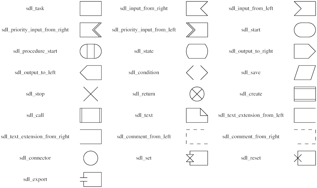
10 - Cluster Attributes

Attributes you can set on subgraph clusters

11 - Edge Attributes

Attributes you can set on graph edges

Examples of edge statements:

edge [name0=val0] sets default edge attribute name0 to val0. Any edge appearing after this inherits the new default attributes.

n1 -> n2 [name1=val1] or n1 \-\- n2 [name1=val1] creates directed or undirected edge between nodes n1 and n2 and sets its attributes according to the optional list and default attributes for edges.

12 - Arrow Shapes

Arrow shapes can be specified and named using the following simple grammar. Terminals are shown in bold font and nonterminals in italics. Literal characters are given in single quotes. Square brackets [ and ] enclose optional items. Vertical bars | separate alternatives.

Grammar

arrowname	:	aname [ aname [ aname [ aname ] ] ]
aname	:	[ modifiers ] shape
modifiers	:	[ 'o' ] [ side ]
side	:	'l'
	\|	'r'
shape	:	box
	\|	crow
	\|	curve
	\|	icurve
	\|	diamond
	\|	dot
	\|	inv
	\|	none
	\|	normal
	\|	tee
	\|	vee

Primitive Shapes

Shape	Image
`box`
`crow`
`curve`
`diamond`
`dot`
`icurve`
`inv`
`none`
`normal`
`tee`
`vee`

Shape Modifiers

As for the modifiers:

'l': Clip the shape, leaving only the part to the left of the edge.
'r': Clip the shape, leaving only the part to the right of the edge.
'o': Use an open (non-filled) version of the shape.

Left and right are defined as those directions determined by looking from the edge towards the point where the arrow "touches" the node.

As an example, the arrow shape lteeoldiamond is parsed as 'l' 'tee' 'o' 'l' 'diamond' and corresponds to the shape:

Note that the first arrow shape specified occurs closest to the node. Subsequent arrow shapes, if specified, occur further from the node. Also, a shape of none uses space, so, for example, the arrowhead nonenormal is not the same as normal.

Not all syntactically legal combinations of modifiers are meaningful or semantically valid. For example, none of the modifiers make any sense with none. The following table indicates which modifiers are allowed with which shapes.

Modifier	`'l'/'r'`	`o`
`box`	✅	✅
`crow`	✅
`curve`	✅
`diamond`	✅	✅
`dot`		✅
`icurve`	✅
`inv`	✅	✅
`none`
`normal`	✅	✅
`tee`	✅
`vee`	✅

This yields 42 different arrow shapes. The optional second, third, fourth shapes can independently be any of the 42, except the last cannot be none as this would create a redundant shape. Thus, there are 41 × 42³ + 41 × 42² + 41 × 42 + 42 = 3,111,696 different combinations.

The following display contains the 42 combinations possible with a single arrow shape. The node attached to the arrow is not drawn but would appear on the right side of the edge.


box	lbox	rbox	obox	olbox	orbox

crow	lcrow	rcrow

diamond	ldiamond	rdiamond	odiamond	oldiamond	ordiamond

dot	odot

inv	linv	rinv	oinv	olinv	orinv

none

normal	lnormal	rnormal	onormal	olnormal	ornormal

tee	ltee	rtee

vee	lvee	rvee

curve	lcurve	rcurve	icurve	licurve	ricurve

13 - Color Names

Color names are resolved in the context of a color scheme. Graphviz currently supports the X11 scheme, the SVG scheme, and the Brewer schemes, with X11 being the default.

Color names are case-insensitive.

In addtition to color names defined by schemes you can also use custom colors.

The Brewer color schemes below are covered by this license.

The X11 color scheme

aliceblue	antiquewhite	antiquewhite1	antiquewhite2	antiquewhite3
antiquewhite4	aqua	aquamarine	aquamarine1	aquamarine2
aquamarine3	aquamarine4	azure	azure1	azure2
azure3	azure4	beige	bisque	bisque1
bisque2	bisque3	bisque4	black	blanchedalmond
blue	blue1	blue2	blue3	blue4
blueviolet	brown	brown1	brown2	brown3
brown4	burlywood	burlywood1	burlywood2	burlywood3
burlywood4	cadetblue	cadetblue1	cadetblue2	cadetblue3
cadetblue4	chartreuse	chartreuse1	chartreuse2	chartreuse3
chartreuse4	chocolate	chocolate1	chocolate2	chocolate3
chocolate4	coral	coral1	coral2	coral3
coral4	cornflowerblue	cornsilk	cornsilk1	cornsilk2
cornsilk3	cornsilk4	crimson	cyan	cyan1
cyan2	cyan3	cyan4	darkblue	darkcyan
darkgoldenrod	darkgoldenrod1	darkgoldenrod2	darkgoldenrod3	darkgoldenrod4
darkgray	darkgreen	darkgrey	darkkhaki	darkmagenta
darkolivegreen	darkolivegreen1	darkolivegreen2	darkolivegreen3	darkolivegreen4
darkorange	darkorange1	darkorange2	darkorange3	darkorange4
darkorchid	darkorchid1	darkorchid2	darkorchid3	darkorchid4
darkred	darksalmon	darkseagreen	darkseagreen1	darkseagreen2
darkseagreen3	darkseagreen4	darkslateblue	darkslategray	darkslategray1
darkslategray2	darkslategray3	darkslategray4	darkslategrey	darkturquoise
darkviolet	deeppink	deeppink1	deeppink2	deeppink3
deeppink4	deepskyblue	deepskyblue1	deepskyblue2	deepskyblue3
deepskyblue4	dimgray	dimgrey	dodgerblue	dodgerblue1
dodgerblue2	dodgerblue3	dodgerblue4	firebrick	firebrick1
firebrick2	firebrick3	firebrick4	floralwhite	forestgreen
fuchsia	gainsboro	ghostwhite	gold	gold1
gold2	gold3	gold4	goldenrod	goldenrod1
goldenrod2	goldenrod3	goldenrod4	gray	gray0
gray1	gray10	gray100	gray11	gray12
gray13	gray14	gray15	gray16	gray17
gray18	gray19	gray2	gray20	gray21
gray22	gray23	gray24	gray25	gray26
gray27	gray28	gray29	gray3	gray30
gray31	gray32	gray33	gray34	gray35
gray36	gray37	gray38	gray39	gray4
gray40	gray41	gray42	gray43	gray44
gray45	gray46	gray47	gray48	gray49
gray5	gray50	gray51	gray52	gray53
gray54	gray55	gray56	gray57	gray58
gray59	gray6	gray60	gray61	gray62
gray63	gray64	gray65	gray66	gray67
gray68	gray69	gray7	gray70	gray71
gray72	gray73	gray74	gray75	gray76
gray77	gray78	gray79	gray8	gray80
gray81	gray82	gray83	gray84	gray85
gray86	gray87	gray88	gray89	gray9
gray90	gray91	gray92	gray93	gray94
gray95	gray96	gray97	gray98	gray99
green	green1	green2	green3	green4
greenyellow	grey	grey0	grey1	grey10
grey100	grey11	grey12	grey13	grey14
grey15	grey16	grey17	grey18	grey19
grey2	grey20	grey21	grey22	grey23
grey24	grey25	grey26	grey27	grey28
grey29	grey3	grey30	grey31	grey32
grey33	grey34	grey35	grey36	grey37
grey38	grey39	grey4	grey40	grey41
grey42	grey43	grey44	grey45	grey46
grey47	grey48	grey49	grey5	grey50
grey51	grey52	grey53	grey54	grey55
grey56	grey57	grey58	grey59	grey6
grey60	grey61	grey62	grey63	grey64
grey65	grey66	grey67	grey68	grey69
grey7	grey70	grey71	grey72	grey73
grey74	grey75	grey76	grey77	grey78
grey79	grey8	grey80	grey81	grey82
grey83	grey84	grey85	grey86	grey87
grey88	grey89	grey9	grey90	grey91
grey92	grey93	grey94	grey95	grey96
grey97	grey98	grey99	honeydew	honeydew1
honeydew2	honeydew3	honeydew4	hotpink	hotpink1
hotpink2	hotpink3	hotpink4	indianred	indianred1
indianred2	indianred3	indianred4	indigo	invis
ivory	ivory1	ivory2	ivory3	ivory4
khaki	khaki1	khaki2	khaki3	khaki4
lavender	lavenderblush	lavenderblush1	lavenderblush2	lavenderblush3
lavenderblush4	lawngreen	lemonchiffon	lemonchiffon1	lemonchiffon2
lemonchiffon3	lemonchiffon4	lightblue	lightblue1	lightblue2
lightblue3	lightblue4	lightcoral	lightcyan	lightcyan1
lightcyan2	lightcyan3	lightcyan4	lightgoldenrod	lightgoldenrod1
lightgoldenrod2	lightgoldenrod3	lightgoldenrod4	lightgoldenrodyellow	lightgray
lightgreen	lightgrey	lightpink	lightpink1	lightpink2
lightpink3	lightpink4	lightsalmon	lightsalmon1	lightsalmon2
lightsalmon3	lightsalmon4	lightseagreen	lightskyblue	lightskyblue1
lightskyblue2	lightskyblue3	lightskyblue4	lightslateblue	lightslategray
lightslategrey	lightsteelblue	lightsteelblue1	lightsteelblue2	lightsteelblue3
lightsteelblue4	lightyellow	lightyellow1	lightyellow2	lightyellow3
lightyellow4	lime	limegreen	linen	magenta
magenta1	magenta2	magenta3	magenta4	maroon
maroon1	maroon2	maroon3	maroon4	mediumaquamarine
mediumblue	mediumorchid	mediumorchid1	mediumorchid2	mediumorchid3
mediumorchid4	mediumpurple	mediumpurple1	mediumpurple2	mediumpurple3
mediumpurple4	mediumseagreen	mediumslateblue	mediumspringgreen	mediumturquoise
mediumvioletred	midnightblue	mintcream	mistyrose	mistyrose1
mistyrose2	mistyrose3	mistyrose4	moccasin	navajowhite
navajowhite1	navajowhite2	navajowhite3	navajowhite4	navy
navyblue	none	oldlace	olive	olivedrab
olivedrab1	olivedrab2	olivedrab3	olivedrab4	orange
orange1	orange2	orange3	orange4	orangered
orangered1	orangered2	orangered3	orangered4	orchid
orchid1	orchid2	orchid3	orchid4	palegoldenrod
palegreen	palegreen1	palegreen2	palegreen3	palegreen4
paleturquoise	paleturquoise1	paleturquoise2	paleturquoise3	paleturquoise4
palevioletred	palevioletred1	palevioletred2	palevioletred3	palevioletred4
papayawhip	peachpuff	peachpuff1	peachpuff2	peachpuff3
peachpuff4	peru	pink	pink1	pink2
pink3	pink4	plum	plum1	plum2
plum3	plum4	powderblue	purple	purple1
purple2	purple3	purple4	rebeccapurple	red
red1	red2	red3	red4	rosybrown
rosybrown1	rosybrown2	rosybrown3	rosybrown4	royalblue
royalblue1	royalblue2	royalblue3	royalblue4	saddlebrown
salmon	salmon1	salmon2	salmon3	salmon4
sandybrown	seagreen	seagreen1	seagreen2	seagreen3
seagreen4	seashell	seashell1	seashell2	seashell3
seashell4	sienna	sienna1	sienna2	sienna3
sienna4	silver	skyblue	skyblue1	skyblue2
skyblue3	skyblue4	slateblue	slateblue1	slateblue2
slateblue3	slateblue4	slategray	slategray1	slategray2
slategray3	slategray4	slategrey	snow	snow1
snow2	snow3	snow4	springgreen	springgreen1
springgreen2	springgreen3	springgreen4	steelblue	steelblue1
steelblue2	steelblue3	steelblue4	tan	tan1
tan2	tan3	tan4	teal	thistle
thistle1	thistle2	thistle3	thistle4	tomato
tomato1	tomato2	tomato3	tomato4	transparent
turquoise	turquoise1	turquoise2	turquoise3	turquoise4
violet	violetred	violetred1	violetred2	violetred3
violetred4	webgray	webgreen	webgrey	webmaroon
webpurple	wheat	wheat1	wheat2	wheat3
wheat4	white	whitesmoke	x11gray	x11green
x11grey	x11maroon	x11purple	yellow	yellow1
yellow2	yellow3	yellow4	yellowgreen

The SVG color scheme

aliceblue	antiquewhite	aqua	aquamarine	azure
beige	bisque	black	blanchedalmond	blue
blueviolet	brown	burlywood	cadetblue	chartreuse
chocolate	coral	cornflowerblue	cornsilk	crimson
cyan	darkblue	darkcyan	darkgoldenrod	darkgray
darkgreen	darkgrey	darkkhaki	darkmagenta	darkolivegreen
darkorange	darkorchid	darkred	darksalmon	darkseagreen
darkslateblue	darkslategray	darkslategrey	darkturquoise	darkviolet
deeppink	deepskyblue	dimgray	dimgrey	dodgerblue
firebrick	floralwhite	forestgreen	fuchsia	gainsboro
ghostwhite	gold	goldenrod	gray	grey
green	greenyellow	honeydew	hotpink	indianred
indigo	ivory	khaki	lavender	lavenderblush
lawngreen	lemonchiffon	lightblue	lightcoral	lightcyan
lightgoldenrodyellow	lightgray	lightgreen	lightgrey	lightpink
lightsalmon	lightseagreen	lightskyblue	lightslategray	lightslategrey
lightsteelblue	lightyellow	lime	limegreen	linen
magenta	maroon	mediumaquamarine	mediumblue	mediumorchid
mediumpurple	mediumseagreen	mediumslateblue	mediumspringgreen	mediumturquoise
mediumvioletred	midnightblue	mintcream	mistyrose	moccasin
navajowhite	navy	oldlace	olive	olivedrab
orange	orangered	orchid	palegoldenrod	palegreen
paleturquoise	palevioletred	papayawhip	peachpuff	peru
pink	plum	powderblue	purple	red
rosybrown	royalblue	saddlebrown	salmon	sandybrown
seagreen	seashell	sienna	silver	skyblue
slateblue	slategray	slategrey	snow	springgreen
steelblue	tan	teal	thistle	tomato
turquoise	violet	wheat	white	whitesmoke
yellow	yellowgreen

Brewer color schemes

accent3 color scheme

1

2

3

accent4 color scheme

1

2

3

4

accent5 color scheme

1

2

3

4

5

accent6 color scheme

1

2

3

4

5

6

accent7 color scheme

1

2

3

4

5

6

7

accent8 color scheme

1

2

3

4

5

6

7

8

blues3 color scheme

1

2

3

blues4 color scheme

1

2

3

4

blues5 color scheme

1

2

3

4

5

blues6 color scheme

1

2

3

4

5

6

blues7 color scheme

1

2

3

4

5

6

7

blues8 color scheme

1

2

3

4

5

6

7

8

blues9 color scheme

1

2

3

4

5

6

7

8

9

brbg10 color scheme

1

2

3

4

5

6

7

8

9

10

brbg11 color scheme

1

2

3

4

5

6

7

8

9

10

11

brbg3 color scheme

1

2

3

brbg4 color scheme

1

2

3

4

brbg5 color scheme

1

2

3

4

5

brbg6 color scheme

1

2

3

4

5

6

brbg7 color scheme

1

2

3

4

5

6

7

brbg8 color scheme

1

2

3

4

5

6

7

8

brbg9 color scheme

1

2

3

4

5

6

7

8

9

bugn3 color scheme

1

2

3

bugn4 color scheme

1

2

3

4

bugn5 color scheme

1

2

3

4

5

bugn6 color scheme

1

2

3

4

5

6

bugn7 color scheme

1

2

3

4

5

6

7

bugn8 color scheme

1

2

3

4

5

6

7

8

bugn9 color scheme

1

2

3

4

5

6

7

8

9

bupu3 color scheme

1

2

3

bupu4 color scheme

1

2

3

4

bupu5 color scheme

1

2

3

4

5

bupu6 color scheme

1

2

3

4

5

6

bupu7 color scheme

1

2

3

4

5

6

7

bupu8 color scheme

1

2

3

4

5

6

7

8

bupu9 color scheme

1

2

3

4

5

6

7

8

9

dark23 color scheme

1

2

3

dark24 color scheme

1

2

3

4

dark25 color scheme

1

2

3

4

5

dark26 color scheme

1

2

3

4

5

6

dark27 color scheme

1

2

3

4

5

6

7

dark28 color scheme

1

2

3

4

5

6

7

8

gnbu3 color scheme

1

2

3

gnbu4 color scheme

1

2

3

4

gnbu5 color scheme

1

2

3

4

5

gnbu6 color scheme

1

2

3

4

5

6

gnbu7 color scheme

1

2

3

4

5

6

7

gnbu8 color scheme

1

2

3

4

5

6

7

8

gnbu9 color scheme

1

2

3

4

5

6

7

8

9

greens3 color scheme

1

2

3

greens4 color scheme

1

2

3

4

greens5 color scheme

1

2

3

4

5

greens6 color scheme

1

2

3

4

5

6

greens7 color scheme

1

2

3

4

5

6

7

greens8 color scheme

1

2

3

4

5

6

7

8

greens9 color scheme

1

2

3

4

5

6

7

8

9

greys3 color scheme

1

2

3

greys4 color scheme

1

2

3

4

greys5 color scheme

1

2

3

4

5

greys6 color scheme

1

2

3

4

5

6

greys7 color scheme

1

2

3

4

5

6

7

greys8 color scheme

1

2

3

4

5

6

7

8

greys9 color scheme

1

2

3

4

5

6

7

8

9

oranges3 color scheme

1

2

3

oranges4 color scheme

1

2

3

4

oranges5 color scheme

1

2

3

4

5

oranges6 color scheme

1

2

3

4

5

6

oranges7 color scheme

1

2

3

4

5

6

7

oranges8 color scheme

1

2

3

4

5

6

7

8

oranges9 color scheme

1

2

3

4

5

6

7

8

9

orrd3 color scheme

1

2

3

orrd4 color scheme

1

2

3

4

orrd5 color scheme

1

2

3

4

5

orrd6 color scheme

1

2

3

4

5

6

orrd7 color scheme

1

2

3

4

5

6

7

orrd8 color scheme

1

2

3

4

5

6

7

8

orrd9 color scheme

1

2

3

4

5

6

7

8

9

paired10 color scheme

1

2

3

4

5

6

7

8

9

10

paired11 color scheme

1

2

3

4

5

6

7

8

9

10

11

paired12 color scheme

1

2

3

4

5

6

7

8

9

10

11

12

paired3 color scheme

1

2

3

paired4 color scheme

1

2

3

4

paired5 color scheme

1

2

3

4

5

paired6 color scheme

1

2

3

4

5

6

paired7 color scheme

1

2

3

4

5

6

7

paired8 color scheme

1

2

3

4

5

6

7

8

paired9 color scheme

1

2

3

4

5

6

7

8

9

pastel13 color scheme

1

2

3

pastel14 color scheme

1

2

3

4

pastel15 color scheme

1

2

3

4

5

pastel16 color scheme

1

2

3

4

5

6

pastel17 color scheme

1

2

3

4

5

6

7

pastel18 color scheme

1

2

3

4

5

6

7

8

pastel19 color scheme

1

2

3

4

5

6

7

8

9

pastel23 color scheme

1

2

3

pastel24 color scheme

1

2

3

4

pastel25 color scheme

1

2

3

4

5

pastel26 color scheme

1

2

3

4

5

6

pastel27 color scheme

1

2

3

4

5

6

7

pastel28 color scheme

1

2

3

4

5

6

7

8

piyg10 color scheme

1

2

3

4

5

6

7

8

9

10

piyg11 color scheme

1

2

3

4

5

6

7

8

9

10

11

piyg3 color scheme

1

2

3

piyg4 color scheme

1

2

3

4

piyg5 color scheme

1

2

3

4

5

piyg6 color scheme

1

2

3

4

5

6

piyg7 color scheme

1

2

3

4

5

6

7

piyg8 color scheme

1

2

3

4

5

6

7

8

piyg9 color scheme

1

2

3

4

5

6

7

8

9

prgn10 color scheme

1

2

3

4

5

6

7

8

9

10

prgn11 color scheme

1

2

3

4

5

6

7

8

9

10

11

prgn3 color scheme

1

2

3

prgn4 color scheme

1

2

3

4

prgn5 color scheme

1

2

3

4

5

prgn6 color scheme

1

2

3

4

5

6

prgn7 color scheme

1

2

3

4

5

6

7

prgn8 color scheme

1

2

3

4

5

6

7

8

prgn9 color scheme

1

2

3

4

5

6

7

8

9

pubu3 color scheme

1

2

3

pubu4 color scheme

1

2

3

4

pubu5 color scheme

1

2

3

4

5

pubu6 color scheme

1

2

3

4

5

6

pubu7 color scheme

1

2

3

4

5

6

7

pubu8 color scheme

1

2

3

4

5

6

7

8

pubu9 color scheme

1

2

3

4

5

6

7

8

9

pubugn3 color scheme

1

2

3

pubugn4 color scheme

1

2

3

4

pubugn5 color scheme

1

2

3

4

5

pubugn6 color scheme

1

2

3

4

5

6

pubugn7 color scheme

1

2

3

4

5

6

7

pubugn8 color scheme

1

2

3

4

5

6

7

8

pubugn9 color scheme

1

2

3

4

5

6

7

8

9

puor10 color scheme

1

2

3

4

5

6

7

8

9

10

puor11 color scheme

1

2

3

4

5

6

7

8

9

10

11

puor3 color scheme

1

2

3

puor4 color scheme

1

2

3

4

puor5 color scheme

1

2

3

4

5

puor6 color scheme

1

2

3

4

5

6

puor7 color scheme

1

2

3

4

5

6

7

puor8 color scheme

1

2

3

4

5

6

7

8

puor9 color scheme

1

2

3

4

5

6

7

8

9

purd3 color scheme

1

2

3

purd4 color scheme

1

2

3

4

purd5 color scheme

1

2

3

4

5

purd6 color scheme

1

2

3

4

5

6

purd7 color scheme

1

2

3

4

5

6

7

purd8 color scheme

1

2

3

4

5

6

7

8

purd9 color scheme

1

2

3

4

5

6

7

8

9

purples3 color scheme

1

2

3

purples4 color scheme

1

2

3

4

purples5 color scheme

1

2

3

4

5

purples6 color scheme

1

2

3

4

5

6

purples7 color scheme

1

2

3

4

5

6

7

purples8 color scheme

1

2

3

4

5

6

7

8

purples9 color scheme

1

2

3

4

5

6

7

8

9

rdbu10 color scheme

1

2

3

4

5

6

7

8

9

10

rdbu11 color scheme

1

2

3

4

5

6

7

8

9

10

11

rdbu3 color scheme

1

2

3

rdbu4 color scheme

1

2

3

4

rdbu5 color scheme

1

2

3

4

5

rdbu6 color scheme

1

2

3

4

5

6

rdbu7 color scheme

1

2

3

4

5

6

7

rdbu8 color scheme

1

2

3

4

5

6

7

8

rdbu9 color scheme

1

2

3

4

5

6

7

8

9

rdgy10 color scheme

1

2

3

4

5

6

7

8

9

10

rdgy11 color scheme

1

2

3

4

5

6

7

8

9

10

11

rdgy3 color scheme

1

2

3

rdgy4 color scheme

1

2

3

4

rdgy5 color scheme

1

2

3

4

5

rdgy6 color scheme

1

2

3

4

5

6

rdgy7 color scheme

1

2

3

4

5

6

7

rdgy8 color scheme

1

2

3

4

5

6

7

8

rdgy9 color scheme

1

2

3

4

5

6

7

8

9

rdpu3 color scheme

1

2

3

rdpu4 color scheme

1

2

3

4

rdpu5 color scheme

1

2

3

4

5

rdpu6 color scheme

1

2

3

4

5

6

rdpu7 color scheme

1

2

3

4

5

6

7

rdpu8 color scheme

1

2

3

4

5

6

7

8

rdpu9 color scheme

1

2

3

4

5

6

7

8

9

rdylbu10 color scheme

1

2

3

4

5

6

7

8

9

10

rdylbu11 color scheme

1

2

3

4

5

6

7

8

9

10

11

rdylbu3 color scheme

1

2

3

rdylbu4 color scheme

1

2

3

4

rdylbu5 color scheme

1

2

3

4

5

rdylbu6 color scheme

1

2

3

4

5

6

rdylbu7 color scheme

1

2

3

4

5

6

7

rdylbu8 color scheme

1

2

3

4

5

6

7

8

rdylbu9 color scheme

1

2

3

4

5

6

7

8

9

rdylgn10 color scheme

1

2

3

4

5

6

7

8

9

10

rdylgn11 color scheme

1

2

3

4

5

6

7

8

9

10

11

rdylgn3 color scheme

1

2

3

rdylgn4 color scheme

1

2

3

4

rdylgn5 color scheme

1

2

3

4

5

rdylgn6 color scheme

1

2

3

4

5

6

rdylgn7 color scheme

1

2

3

4

5

6

7

rdylgn8 color scheme

1

2

3

4

5

6

7

8

rdylgn9 color scheme

1

2

3

4

5

6

7

8

9

reds3 color scheme

1

2

3

reds4 color scheme

1

2

3

4

reds5 color scheme

1

2

3

4

5

reds6 color scheme

1

2

3

4

5

6

reds7 color scheme

1

2

3

4

5

6

7

reds8 color scheme

1

2

3

4

5

6

7

8

reds9 color scheme

1

2

3

4

5

6

7

8

9

set13 color scheme

1

2

3

set14 color scheme

1

2

3

4

set15 color scheme

1

2

3

4

5

set16 color scheme

1

2

3

4

5

6

set17 color scheme

1

2

3

4

5

6

7

set18 color scheme

1

2

3

4

5

6

7

8

set19 color scheme

1

2

3

4

5

6

7

8

9

set23 color scheme

1

2

3

set24 color scheme

1

2

3

4

set25 color scheme

1

2

3

4

5

set26 color scheme

1

2

3

4

5

6

set27 color scheme

1

2

3

4

5

6

7

set28 color scheme

1

2

3

4

5

6

7

8

set310 color scheme

1

2

3

4

5

6

7

8

9

10

set311 color scheme

1

2

3

4

5

6

7

8

9

10

11

set312 color scheme

1

2

3

4

5

6

7

8

9

10

11

12

set33 color scheme

1

2

3

set34 color scheme

1

2

3

4

set35 color scheme

1

2

3

4

5

set36 color scheme

1

2

3

4

5

6

set37 color scheme

1

2

3

4

5

6

7

set38 color scheme

1

2

3

4

5

6

7

8

set39 color scheme

1

2

3

4

5

6

7

8

9

spectral10 color scheme

1

2

3

4

5

6

7

8

9

10

spectral11 color scheme

1

2

3

4

5

6

7

8

9

10

11

spectral3 color scheme

1

2

3

spectral4 color scheme

1

2

3

4

spectral5 color scheme

1

2

3

4

5

spectral6 color scheme

1

2

3

4

5

6

spectral7 color scheme

1

2

3

4

5

6

7

spectral8 color scheme

1

2

3

4

5

6

7

8

spectral9 color scheme

1

2

3

4

5

6

7

8

9

ylgn3 color scheme

1

2

3

ylgn4 color scheme

1

2

3

4

ylgn5 color scheme

1

2

3

4

5

ylgn6 color scheme

1

2

3

4

5

6

ylgn7 color scheme

1

2

3

4

5

6

7

ylgn8 color scheme

1

2

3

4

5

6

7

8

ylgn9 color scheme

1

2

3

4

5

6

7

8

9

ylgnbu3 color scheme

1

2

3

ylgnbu4 color scheme

1

2

3

4

ylgnbu5 color scheme

1

2

3

4

5

ylgnbu6 color scheme

1

2

3

4

5

6

ylgnbu7 color scheme

1

2

3

4

5

6

7

ylgnbu8 color scheme

1

2

3

4

5

6

7

8

ylgnbu9 color scheme

1

2

3

4

5

6

7

8

9

ylorbr3 color scheme

1

2

3

ylorbr4 color scheme

1

2

3

4

ylorbr5 color scheme

1

2

3

4

5

ylorbr6 color scheme

1

2

3

4

5

6

ylorbr7 color scheme

1

2

3

4

5

6

7

ylorbr8 color scheme

1

2

3

4

5

6

7

8

ylorbr9 color scheme

1

2

3

4

5

6

7

8

9

ylorrd3 color scheme

1

2

3

ylorrd4 color scheme

1

2

3

4

ylorrd5 color scheme

1

2

3

4

5

ylorrd6 color scheme

1

2

3

4

5

6

ylorrd7 color scheme

1

2

3

4

5

6

7

ylorrd8 color scheme

1

2

3

4

5

6

7

8

ylorrd9 color scheme

1

2

3

4

5

6

7

8

9

ColorBrewer License

Apache-Style Software License for ColorBrewer software and ColorBrewer Color Schemes, Version 1.1

Redistribution and use in source and binary forms, with or without modification, are permitted provided that the following conditions are met:

Redistributions as source code must retain the above copyright notice, this list of conditions and the following disclaimer.
The end-user documentation included with the redistribution, if any, must include the following acknowledgment:

This product includes color specifications and designs developed by Cynthia Brewer (http://colorbrewer.org/).

Alternately, this acknowledgment may appear in the software itself, if and wherever such third-party acknowledgments normally appear.
The name "ColorBrewer" must not be used to endorse or promote products derived from this software without prior written permission. For written permission, please contact Cynthia Brewer at cbrewer@psu.edu.
Products derived from this software may not be called "ColorBrewer", nor may "ColorBrewer" appear in their name, without prior written permission of Cynthia Brewer.

THIS SOFTWARE IS PROVIDED "AS IS" AND ANY EXPRESSED OR IMPLIED WARRANTIES, INCLUDING, BUT NOT LIMITED TO, THE IMPLIED WARRANTIES OF MERCHANTABILITY AND FITNESS FOR A PARTICULAR PURPOSE ARE DISCLAIMED. IN NO EVENT SHALL CYNTHIA BREWER, MARK HARROWER, OR THE PENNSYLVANIA STATE UNIVERSITY BE LIABLE FOR ANY DIRECT, INDIRECT, INCIDENTAL, SPECIAL, EXEMPLARY, OR CONSEQUENTIAL DAMAGES (INCLUDING, BUT NOT LIMITED TO, PROCUREMENT OF SUBSTITUTE GOODS OR SERVICES; LOSS OF USE, DATA, OR PROFITS; OR BUSINESS INTERRUPTION) HOWEVER CAUSED AND ON ANY THEORY OF LIABILITY, WHETHER IN CONTRACT, STRICT LIABILITY, OR TORT (INCLUDING NEGLIGENCE OR OTHERWISE) ARISING IN ANY WAY OUT OF THE USE OF THIS SOFTWARE, EVEN IF ADVISED OF THE POSSIBILITY OF SUCH DAMAGE.

14 - Character Entities

This reference is generated from: http://www.w3.org/TR/html4/sgml/entities.html using the entities.tcl demo program from the graphviz distribution.

See Character Encodings.

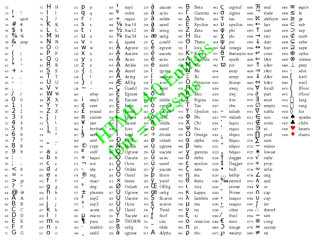
15 - Library Usage

Using Graphviz as a library

Library User guides:

Graphviz C Libraries

PDF manuals:

Sample C Programs using Graphviz as a Library:

Documentation

1 - DOT Language

Subgraphs and Clusters

Lexical and Semantic Notes

Character encodings

2 - Command Line

Flags

-Gname[=value]

-Nname[=value]

-Ename[=value]

-Klayout

-Tformat[:renderer[:formatter]]

-V

-llibrary

-n[num]

-ooutfile

-O

-P

-q

-s[scale]

-v

-x

-y

-?

Environment Variables

GDFONTPATH

DOTFONTPATH

SERVER_NAME

GVBINDIR

2.1 - acyclic

2.2 - bcomps

2.3 - ccomps

2.4 - cluster

2.5 - diffimg

2.6 - dijkstra

2.7 - dotty

2.8 - edgepaint

2.9 - gc

2.10 - gml2gv

2.11 - graphml2gv

2.12 - gv2gxl

2.13 - gvcolor

2.14 - gvedit

2.15 - gvgen

2.16 - gvmap

2.17 - gvpack

2.18 - gvpr

2.19 - gxl2gv

2.20 - lefty

2.21 - lneato

2.22 - mingle

2.23 - mm2gv

2.24 - nop

2.25 - sccmap

2.26 - smyrna

2.27 - tred

2.28 - unflatten

2.29 - vimdot

3 - Layout Engines

3.1 - dot

Attributes for dot features

3.2 - neato

Attributes for neato features

3.3 - fdp

Attributes for fdp features

3.4 - sfdp

Attributes for sfdp features

3.5 - circo

Attributes for circo features

3.6 - twopi

Attributes for twopi features

3.7 - nop

3.8 - nop2

3.9 - osage

3.10 - patchwork

Attributes for patchwork features

3.11 - Writing Layout Plugins

Layout

Cleanup

Automake Configuration

`-G`name[=value]

`-N`name[=value]

`-E`name[=value]

`-K`layout

`-T`format[:renderer[:formatter]]

`-V`

`-l`library

`-n`[num]

`-o`outfile

`-O`

`-P`

`-q`

`-s`[scale]

`-v`

`-x`

`-y`

`-?`

`GDFONTPATH`

`DOTFONTPATH`

`SERVER_NAME`

`GVBINDIR`